Lecture 3: Sea-floor depth, age, and heat flow

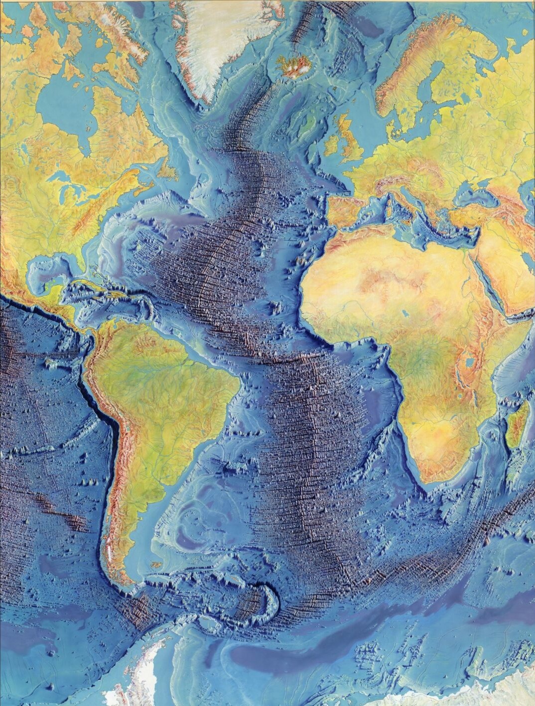
• Mid ocean ridges and the topography of the sea-floor
  • Heat transport in the Earth
  • Boundary layer model
  • Plate model
• How do we map the seafloor today?
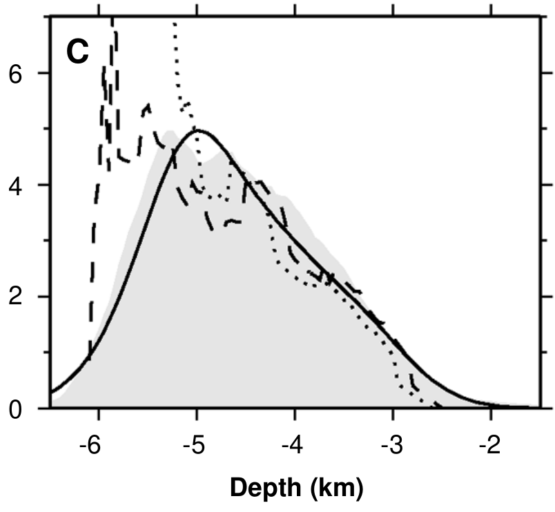
  • Stochastic reheating model

We acknowledge and respect the lək̓ʷəŋən peoples on whose traditional territory the university stands and the Songhees, Esquimalt and W̱SÁNEĆ peoples whose historical relationships with the land continue to this day.

The lithosphere

We can image the crust pretty well, but not the base of the lithosphere

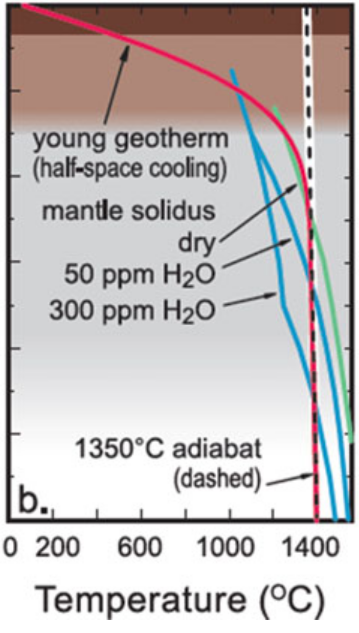
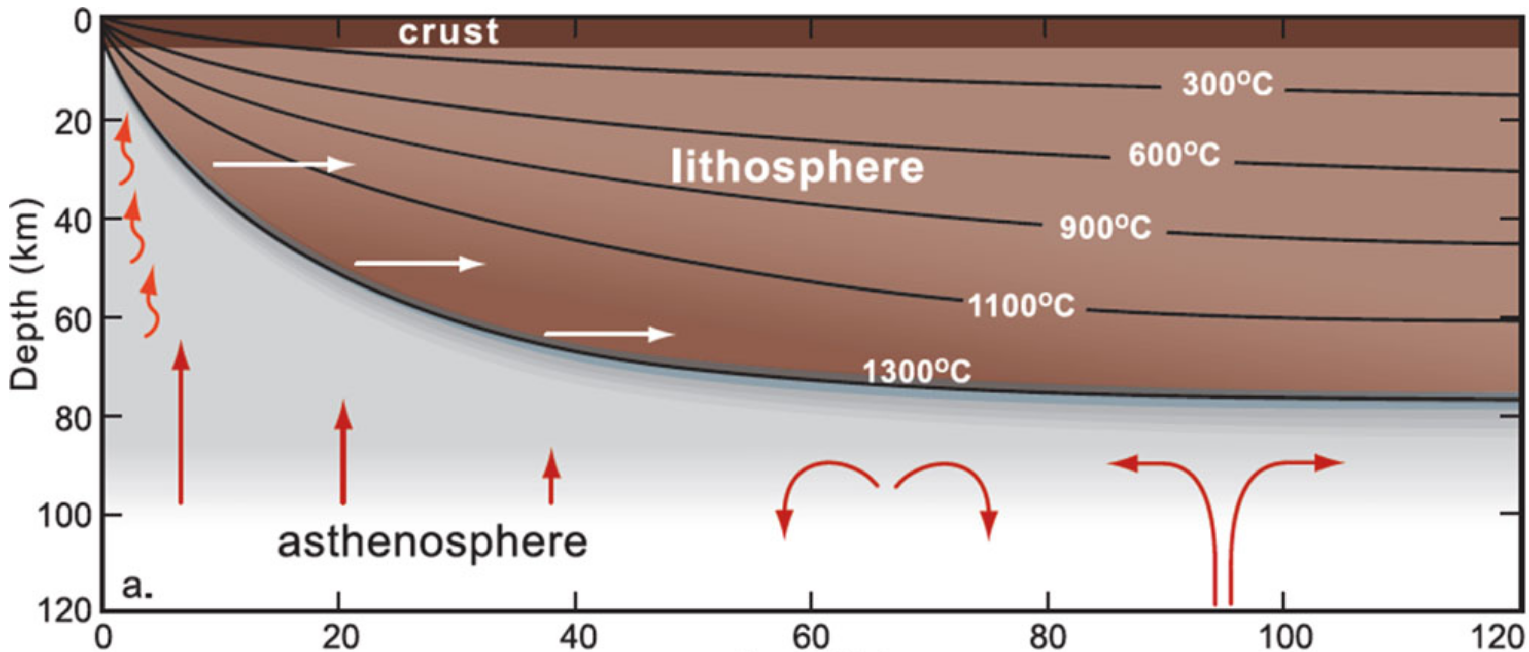
Temperature pr ofile of Earth's lithosphere and upper asthenosphere (sketch first)

Temperature profile of Earth's lithosphere and upper asthenosphere (sketch first)

Temperature profile of Earth's lithosphere and upper asthenosphere (sketch first)

Heat flux (Fourier's law)

The differential form of Fourier's law of thermal conduction shows that the local heat flux density, $q$, is equal to the product of thermal conductivity, $k$, and the negative local temperature gradient, ${\partial T}/{\partial x}$. The heat flux density is the amount of energy that flows through a unit area per unit time.

$$ q = -k \frac{\partial T}{\partial x} $$

How does temperature change over time through conduction?

The diffusion equation: $$ \frac{\partial T}{\partial t} = \frac{\partial q}{\partial x} $$

$$ \frac{\partial T}{\partial t} = -k \frac{\partial^2 T}{\partial x^2} $$

• draw box with flux in and out
• show discrete form where dh/dt = (q1-q2)
• show heat equation (diffusion)

Heat flux (Fourier's law)

• Using your intuition of diffusion, draw some sketches showing:
  • Temperature profile of asthenosphere (1400 $^\circ$C) instantly brought to the surface (0 $^\circ$C)
  • Temperature profile of this asthenosphere after an intermediate time
  • Temperature profile of this asthenosphere after a long time

How does heat flux, $q$, change at the surface in each instance?

• Draw a sketch of a mid ocean ridge, annotating the crust, the lithosphere-asthenosphere boundary, and a few isotherms (temperature contours)

Heat flux observations

Dashed line represents a simple conductive cooling model. What patterns to the misfit do you see?

Younger sea-floor has hydrothermal cooling (lower heat flux than expected). We'll take a closer look at the old sea-floor problem soon!

Under what conditions do you get a steady state solution to the heat equation? What does this solution look like? (draw a profile)

Heat flux observations

Dashed line represents a simple conductive cooling model. What patterns to the misfit do you see?

Younger sea-floor has hydrothermal cooling (lower heat flux than expected). We'll take a closer look at the old sea-floor problem soon!

Under what conditions do you get a steady state solution to the heat equation? What does this solution look like? (draw a profile)

Heat flux observations

Dashed line represents a simple conductive cooling model. What patterns to the misfit do you see?

Younger sea-floor has hydrothermal cooling (lower heat flux than expected). We'll take a closer look at the old sea-floor problem soon!

Under what conditions do you get a steady state solution to the heat equation? What does this solution look like? (draw a profile)

Heat flux observations

Dashed line represents a simple conductive cooling model. What patterns to the misfit do you see?

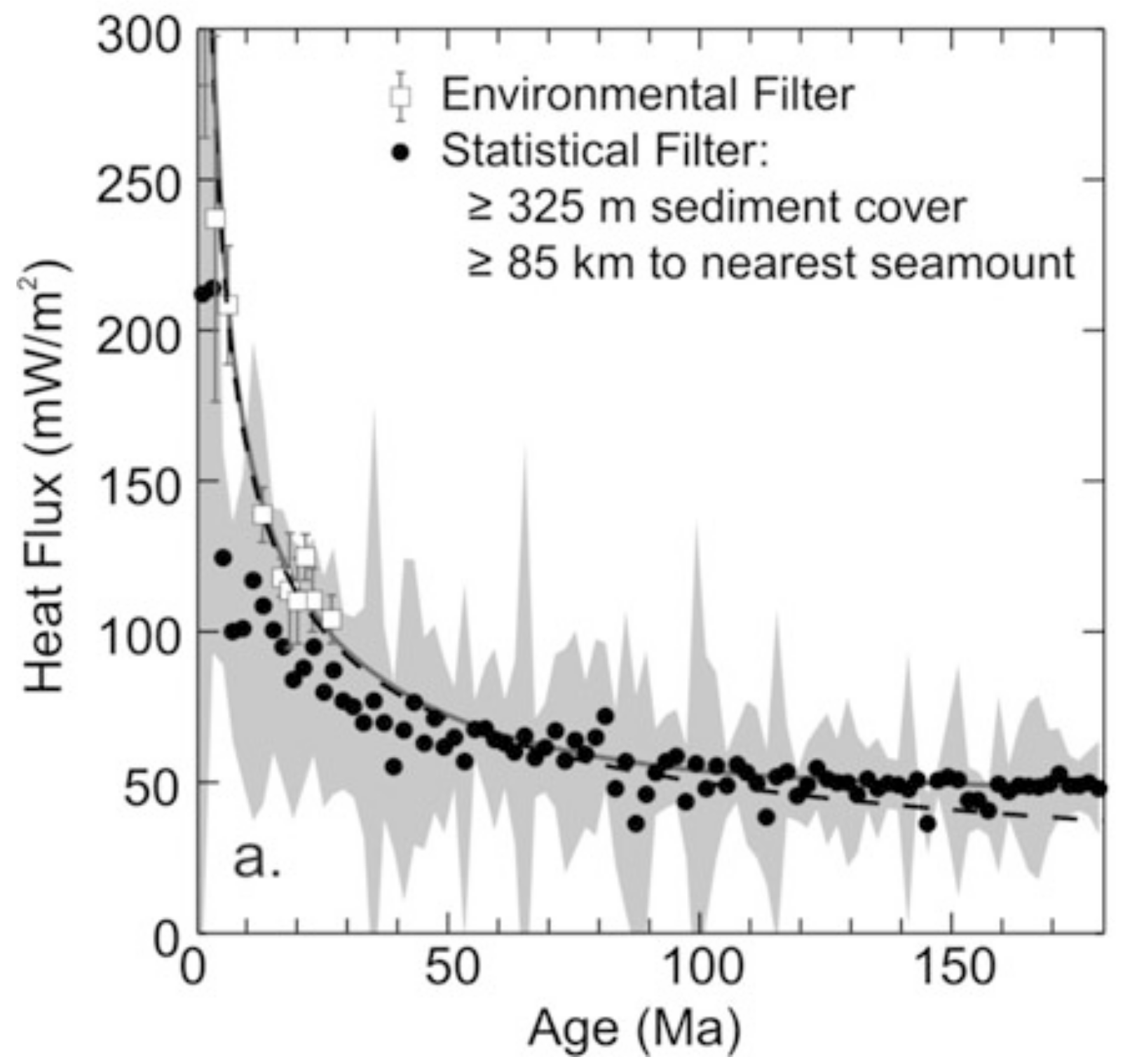
Younger sea-floor has hydrothermal cooling (lower heat flux than expected). We'll take a closer look at the old sea-floor problem soon!

Under what conditions do you get a steady state solution to the heat equation? What does this solution look like? (draw a profile)

Boundary Layer Model (cooling of an infinite half-space)

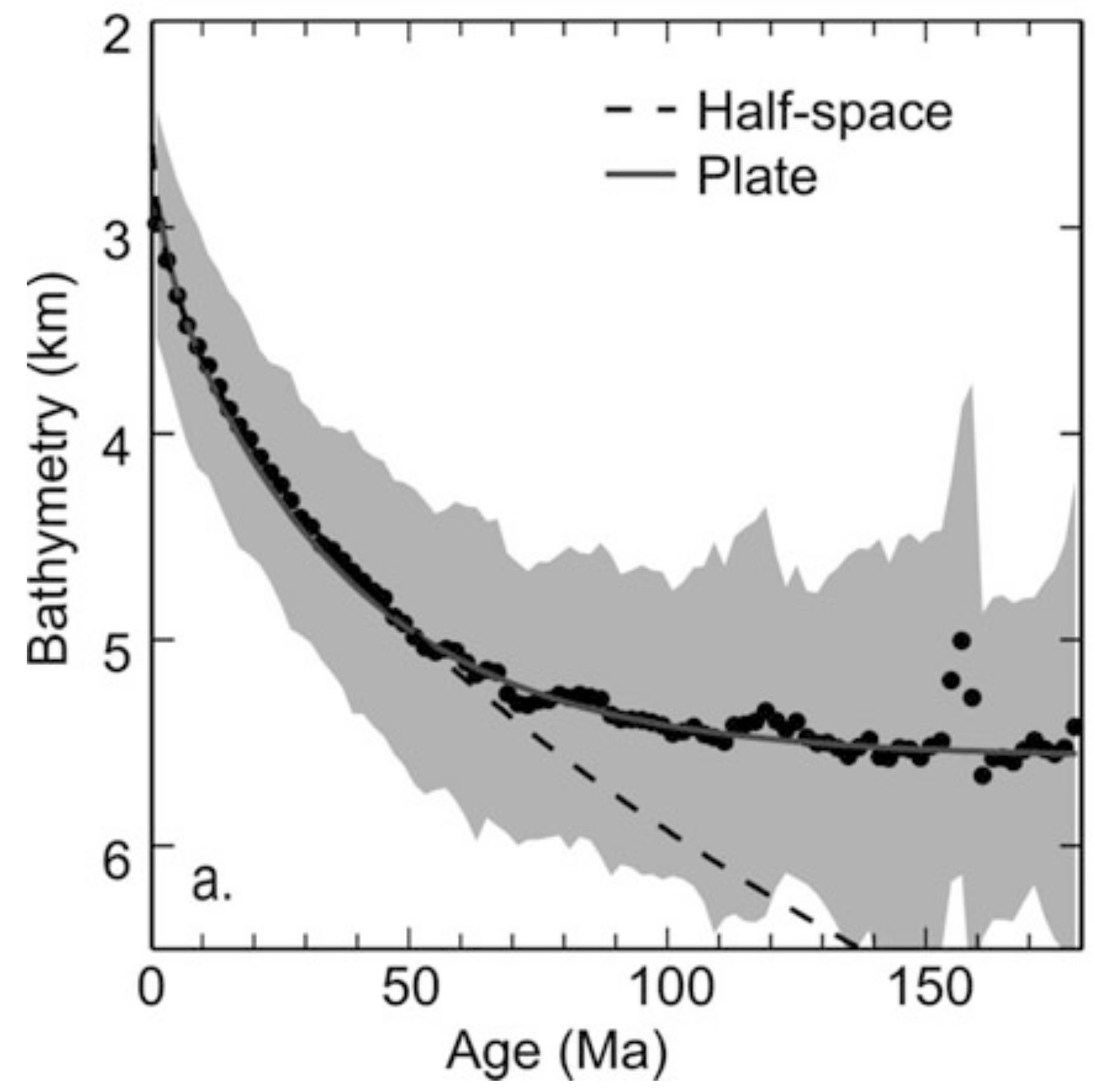
Boundary Layer Model (cooling of an infinite half-space)

If the sea-floor gets deeper away from a mid-ocean ridge, is the lithosphere density high or lower than the asthenosphere?

• Calculate the thickness of the lithosphere
  • at 0 Ma (3 km bathymetry)
  • at 20 Ma (4 km bathymetry)
  • at 50 Ma (5 km bathymetry)

• Using the following densities:
  • Cool peridotite (lithosphere): 3400 kg/m$^3$
  • Hot peridotite (asthenosphere): 3300 kg/m$^3$
  • Water: 1000 kg/m$^3$

Boundary Layer Model (cooling of an infinite half-space)

If the sea-floor gets deeper away from a mid-ocean ridge, is the lithosphere density high or lower than the asthenosphere?

• Calculate the thickness of the lithosphere
  • at 0 Ma (3 km bathymetry)
  • at 20 Ma (4 km bathymetry)
  • at 50 Ma (5 km bathymetry)

• Using the following densities:
  • Cool peridotite (lithosphere): 3400 kg/m$^3$
  • Hot peridotite (asthenosphere): 3300 kg/m$^3$
  • Water: 1000 kg/m$^3$

Boundary Layer Model (cooling of an infinite half-space)

The dashed line is the predicted topography of the sea-floor using the diffusion equation and measured thermal conductivities of mantle material. Why do you think the model fails for older crust?

The denser lithosphere thickness stops increasing (maximum plate thickness). Why?

Plate model

"A more realistic model is developed here, based on the idea that the thermal structure of the plate becomes unstable and leads to the development of small-scale convection. Convective heat transport then supplies the heat flux needed to match the observations rather than an artificial constant temperature boundary condition. The temperature dependence of the rheology is represented in a simple manner. Below a given temperature the material is assumed to move rigidly, defining an upper mechanical boundary layer. Beneath this rigid layer, where the temperatures are greater, the material is assumed to have a constant Newtonian viscosity. The part of the viscous region where there are significant vertical temperature gradients, immediately below the mechanical boundary layer, forms a thermal boundary layer. As the plate cools, both the mechanical and thermal boundary layers increase in thickness. A local critical Rayleigh number criterion is used to test the stability of the thermal boundary layer. On this basis a convective instability is predicted, its occurrence coinciding with the breakdown of the linear dependence of the depth of the ocean floor on the square root of age." Parsons and McKenzie, Mantle Convection and the Thermal Structure of the Plates, 1978

Plate model

"A more realistic model is developed here, based on the idea that the thermal structure of the plate becomes unstable and leads to the development of small-scale convection. Convective heat transport then supplies the heat flux needed to match the observations rather than an artificial constant temperature boundary condition. The temperature dependence of the rheology is represented in a simple manner. Below a given temperature the material is assumed to move rigidly, defining an upper mechanical boundary layer. Beneath this rigid layer, where the temperatures are greater, the material is assumed to have a constant Newtonian viscosity. The part of the viscous region where there are significant vertical temperature gradients, immediately below the mechanical boundary layer, forms a thermal boundary layer. As the plate cools, both the mechanical and thermal boundary layers increase in thickness. A local critical Rayleigh number criterion is used to test the stability of the thermal boundary layer. On this basis a convective instability is predicted, its occurrence coinciding with the breakdown of the linear dependence of the depth of the ocean floor on the square root of age." Parsons and McKenzie, Mantle Convection and the Thermal Structure of the Plates, 1978

Plate model

"A more realistic model is developed here, based on the idea that the thermal structure of the plate becomes unstable and leads to the development of small-scale convection. Convective heat transport then supplies the heat flux needed to match the observations rather than an artificial constant temperature boundary condition. The temperature dependence of the rheology is represented in a simple manner. Below a given temperature the material is assumed to move rigidly, defining an upper mechanical boundary layer. Beneath this rigid layer, where the temperatures are greater, the material is assumed to have a constant Newtonian viscosity. The part of the viscous region where there are significant vertical temperature gradients, immediately below the mechanical boundary layer, forms a thermal boundary layer. As the plate cools, both the mechanical and thermal boundary layers increase in thickness. A local critical Rayleigh number criterion is used to test the stability of the thermal boundary layer. On this basis a convective instability is predicted, its occurrence coinciding with the breakdown of the linear dependence of the depth of the ocean floor on the square root of age." Parsons and McKenzie, Mantle Convection and the Thermal Structure of the Plates, 1978

As the plate cools, both the mechanical and thermal boundary layers increase in thickness

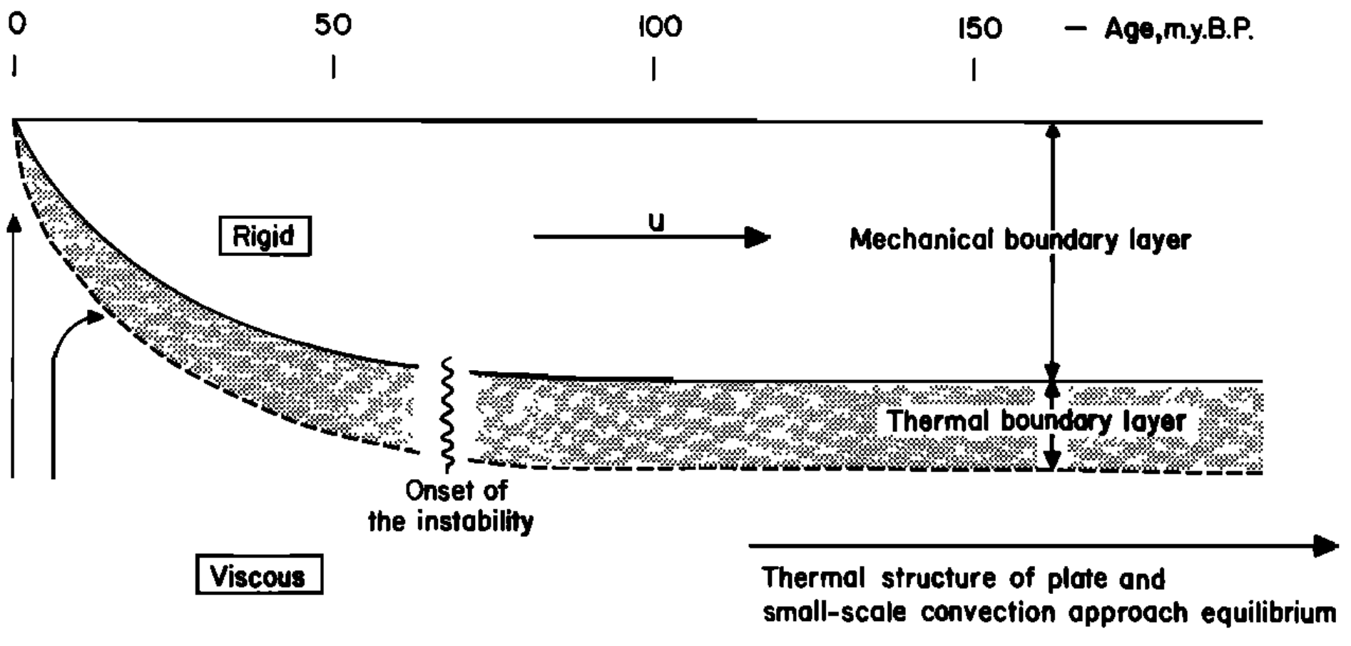
What exactly is this thermal boundary layer?

"A local critical Rayleigh number criterion is used to test the stability of the thermal boundary layer. On this basis a convective instability is predicted, its occurrence coinciding with the breakdown of the linear dependence of the depth of the ocean floor on the square root of age." Parsons and McKenzie, Mantle Convection and the Thermal Structure of the Plates, 1978

• Rayleigh number describes how heat is transferred in a material with non-uniform density (often due to temperature differences)
  • Low Rayleigh number: conduction
  • High Rayleigh number: convection

Parsons and McKenzie are specifically describing a layer near the lithosphere-asthenosphere boundary where the combined viscosity contrasts (mechanical) and temperature contrasts lead to small scale convection.

Thermal boundary layers

What exactly is this thermal boundary layer?

Thermal boundary layers

What exactly is this thermal boundary layer?

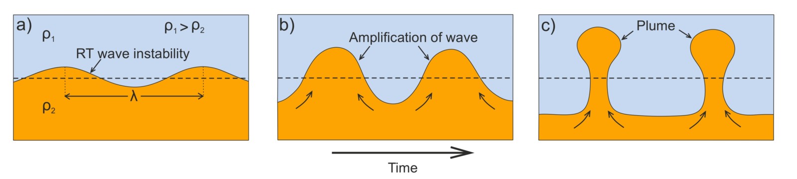
Thermal boundary layers

What exactly is this thermal boundary layer?

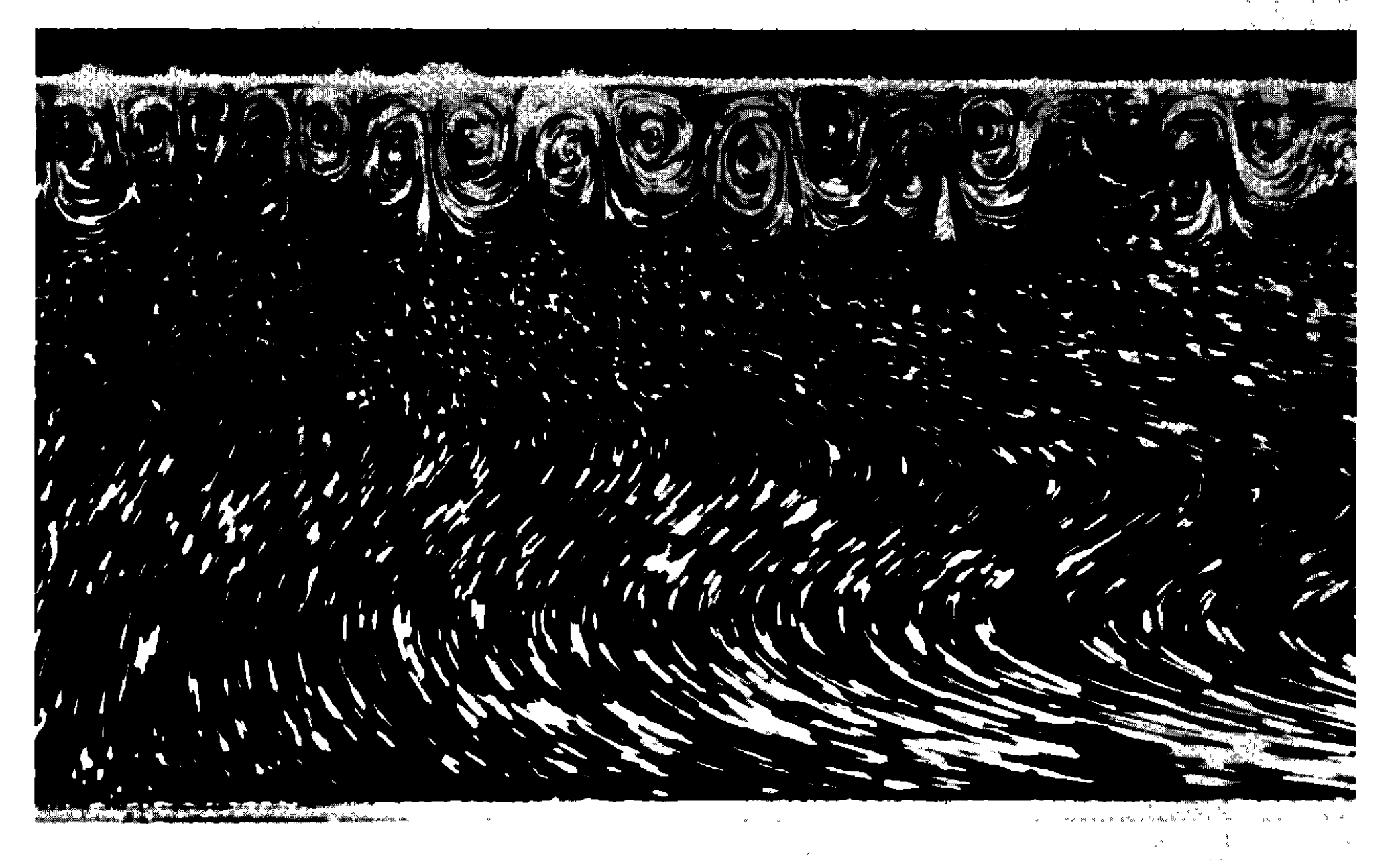
Thermal boundary layers

How does this thermal instability effect plate (lithosphere) thicknesses?

Does convection increase or decrease heat flux rates?

Higher heat flux to the base of the lithosphere after the instability forms, resulting in a near constant temperature at the base of the lithosphere (the instability delivers heat as fast as conductive cooling above can remove it, a steady state).

Recall our drawings of thermal profiles earlier, how does a fixed boundary condition at 100 km change the temperature profile in the lithosphere?

Mapping the sea-floor

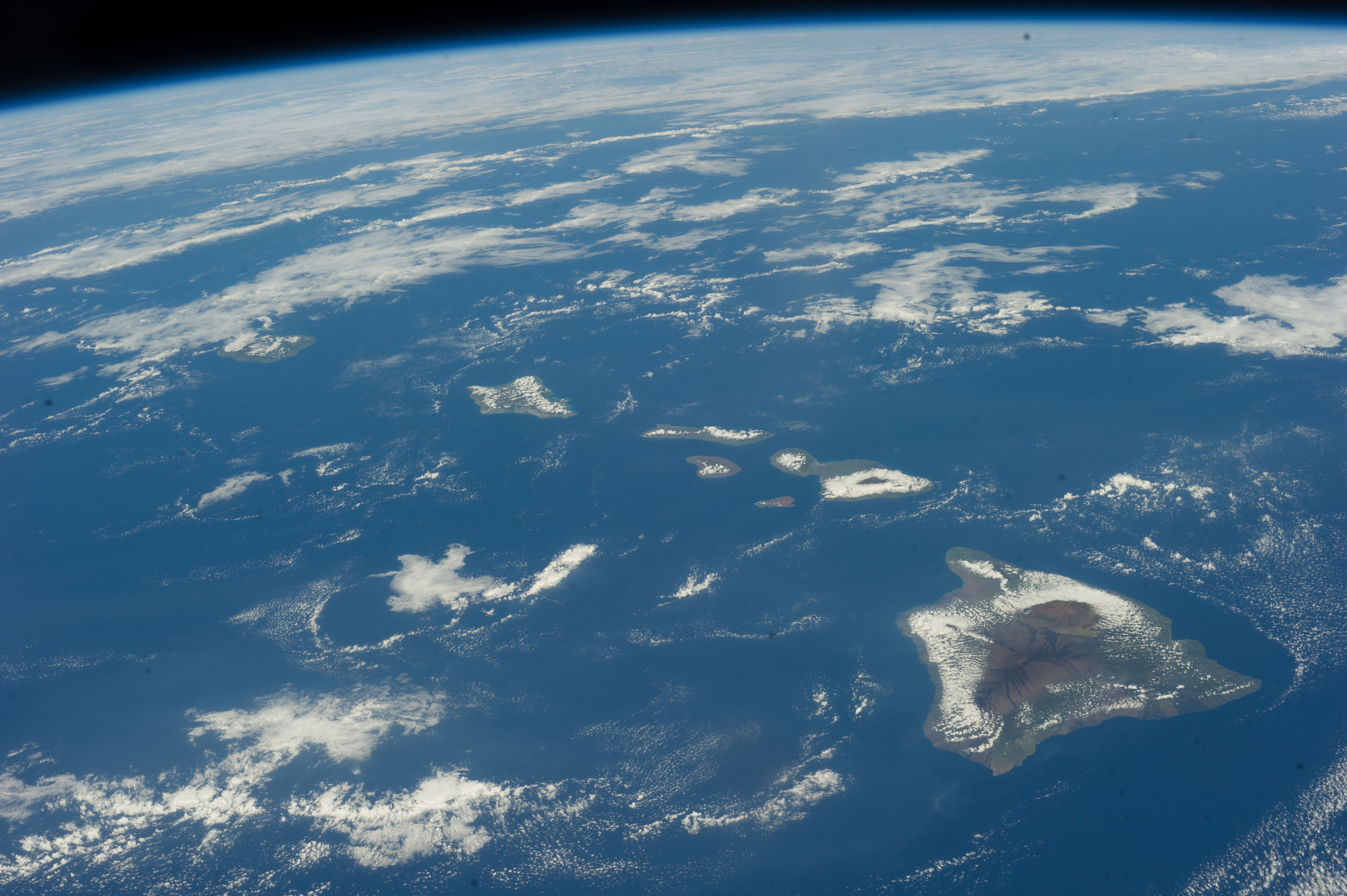
How do we map the bathymetry of the sea-floor?

Mapping the sea-floor

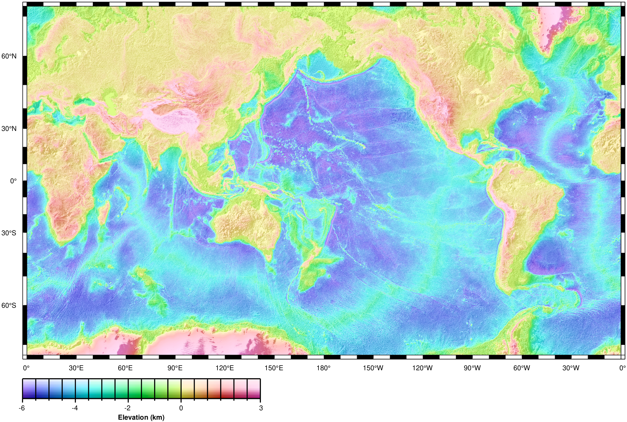
How do we map the bathymetry of the sea-floor?

• A combination of:
  • Depth Soundings
  • Satellite Altimetry

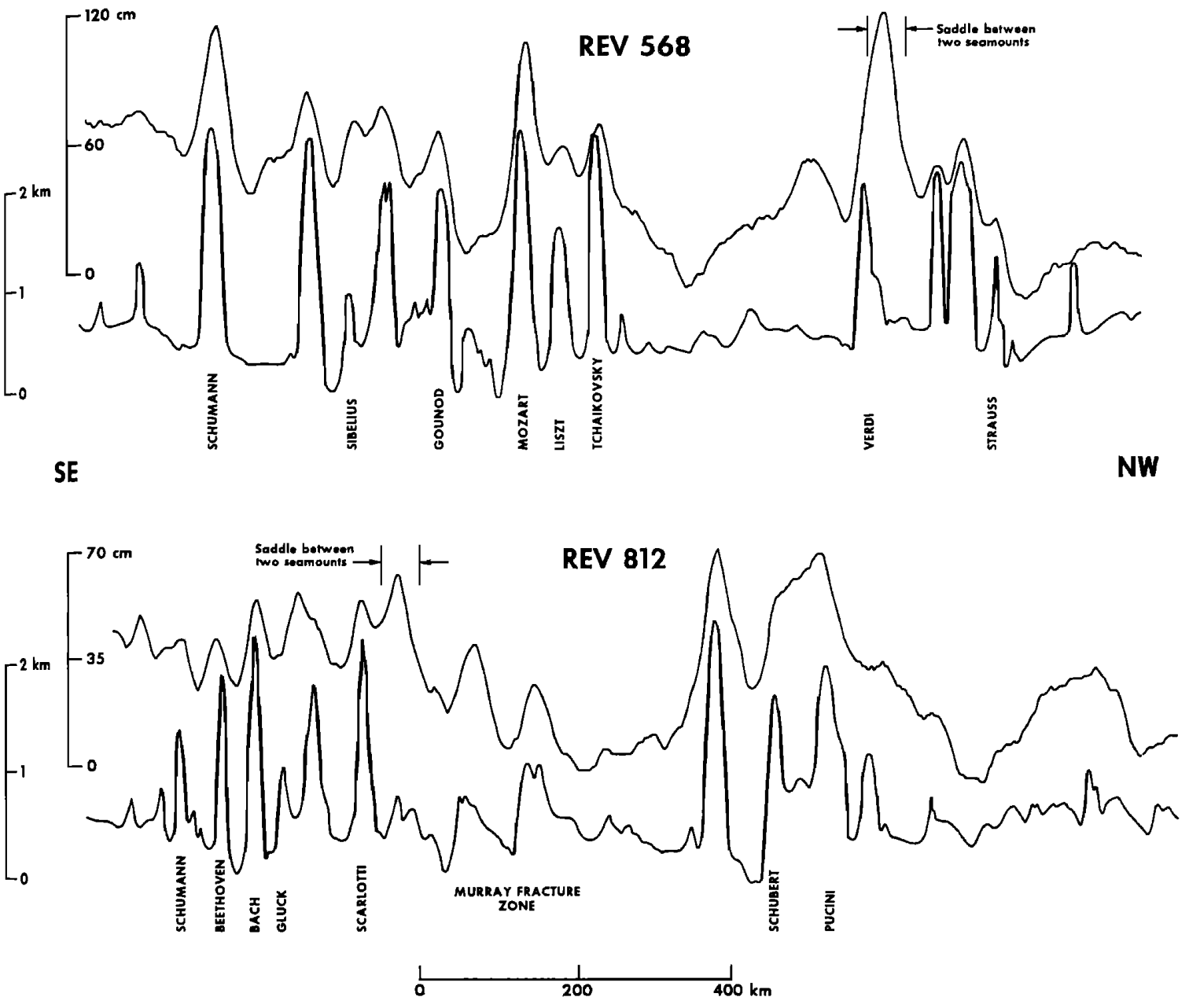
Bathymetric Prediction From SEASAT Altimeter Data (Dixon et al. 1983)

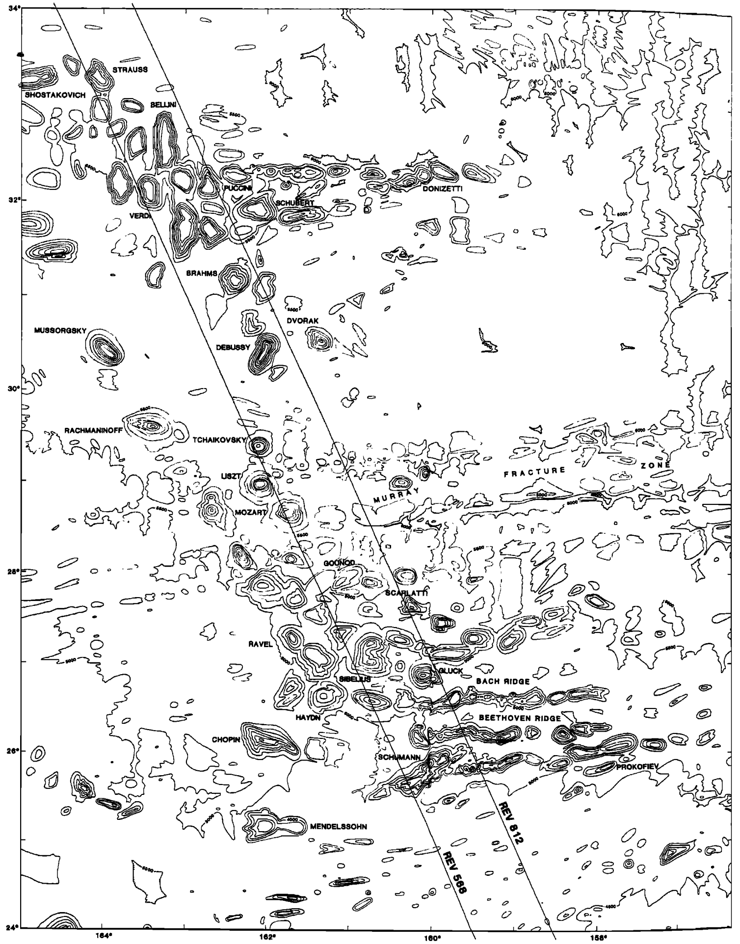
Bathymetric Prediction From SEASAT Altimeter Data (Dixon et al. 1983)

Gravitational potential

Gravitational potential is the the work (energy transferred) per unit mass that would be needed to move an object to that point from a distance infinitely far away. Recall that: $$ \mathrm{work = force~\times~displacement} $$

The force of gravity is constant along an equipotential surface (in other words, the acceleration of a unit mass is the same). One such surface on Earth is commonly referred to as the geoid. What is the geoid?

If the Earth is isostatically compensated, why does the geoid (sea-surface) vary?

• Consider (and sketch) equipotential surfaces:
  • very far from Earth (treat Earth as a point mass)
  • On Earth's surface place a high density block:
    • Draw the 3 equipotential surfaces approaching the block from the upper atmosphere

• variations are small amplitude
• due to lateral differences in density
• high wavelength variations are due to difference deep in the Earth
• low wavelength variations are due to differences near the surface of the Earth

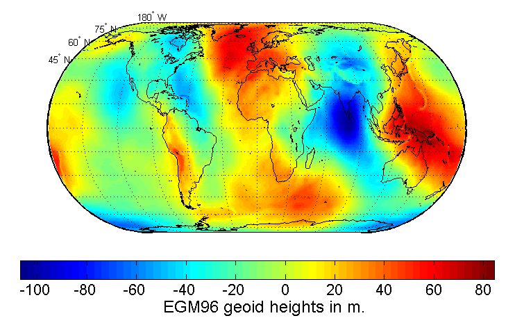
If the Earth is isostatically compensated, why does the geoid (sea-surface) vary?

• Consider (and sketch) equipotential surfaces:
  • very far from Earth (treat Earth as a point mass)
  • On Earth's surface place a high density block:
    • Draw the 3 equipotential surfaces approaching the block from the upper atmosphere

• variations are small amplitude
• due to lateral differences in density
• high wavelength variations are due to difference deep in the Earth
• low wavelength variations are due to differences near the surface of the Earth

Mapping the sea-floor

• Altimetry data decomposed into high frequency (low wavelength) and low frequency (high wavelength) spectral components
• Low frequency components are combined with ship soundings to estimate deeper Earth density structures
• High frequency components are used to interpolate between soundings, assuming deep structure constant
• High frequency components are used to resolve very shallow density contrasts (such as sea-mounts)

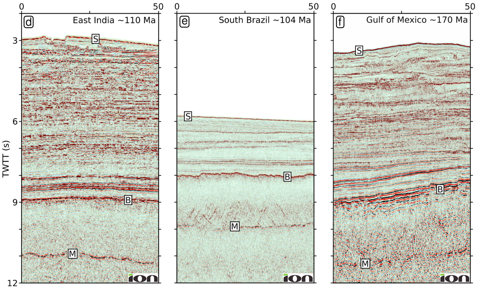
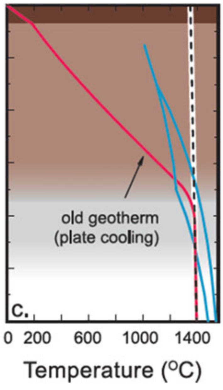
Returning to the plate model and old oceanic lithosphere

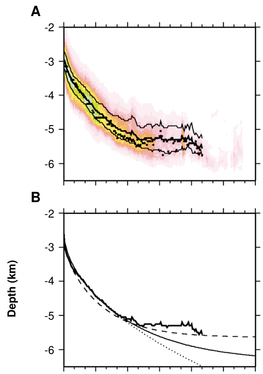
Returning to the plate model and old oceanic lithosphere