Lecture 3: Discussion of Kenyon and Turcotte (1985)

Lecture 3: Discussion of Kenyon and Turcotte (1985)

• working pairs will be selected at random to lead discussion on different parts of the paper
• you can use the board to talk through concepts
• if a slide heading is in blue, then the picked group should take the lead (esp. questions in bold)
• if a slide heading is in red, then I will take the lead
• sections to be discussed:
  • Introduction and Motivation (or, why was this paper written)?
  • Setting-up the model: applying the diffusion equation (why is this an appropriate approach?)
  • Making the model: getting to an equation for delta morphology
  • Using the model: comparing to real world

import random
def pick_group(class_list):
    if len(class_list)>0:
        picked=random.sample(class_list,2)
        [class_list.remove(p) for p in picked]
        print(' and '.join(picked))
    else:
        picked=[]
    return class_list,picked

Introduction and motivation

What is being shown here, and how does it relate to the paper topic?

• foresets, predominantly bedload, lying at angle of repose
• grade into bottom sets, suspended load
• two different processes, actions of individual particles
• but real deltas often much shallower than angle or repose
• also hard to tell difference between bottom sets and fore sets

class_list = ['Kai','Stacey','Grace','Liam','Matteo','Matthew','Noa','Izzy','Felix','Rhys','Andrea','Kristyn']
class_list,picked=pick_group(class_list)

Introduction and motivation

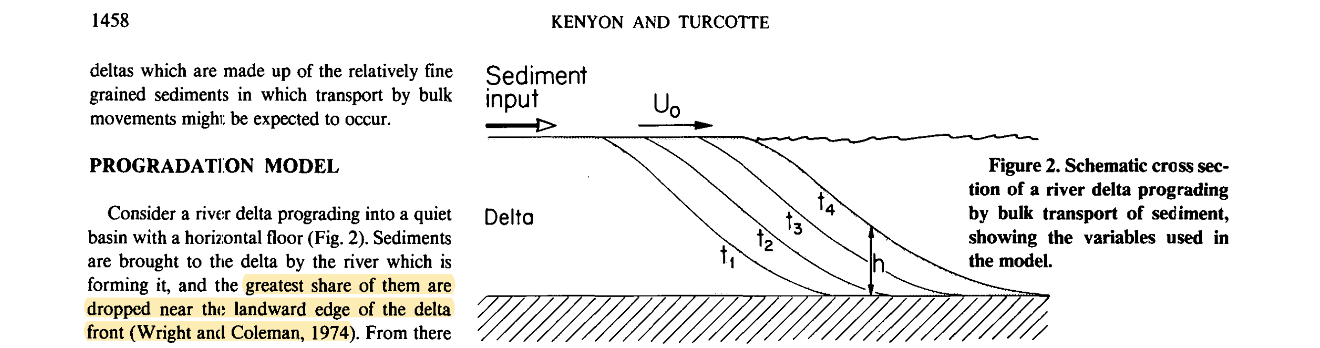
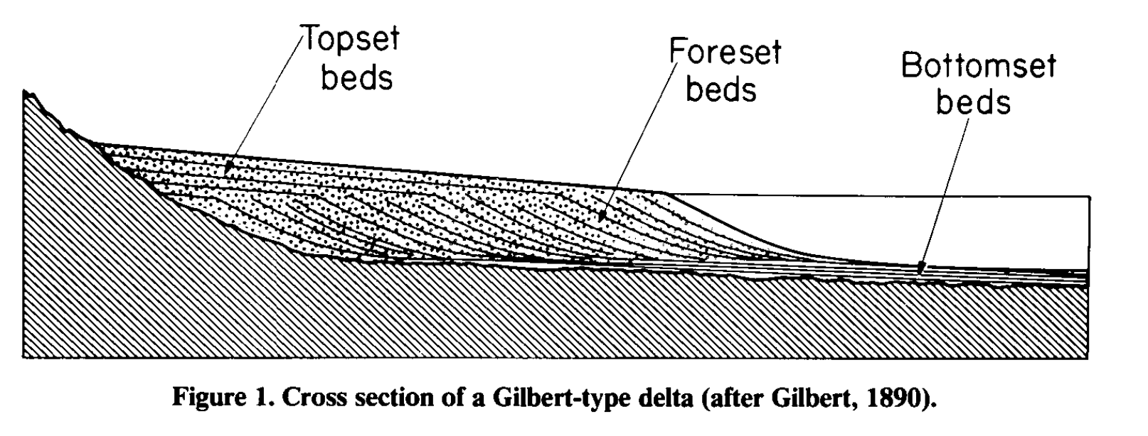
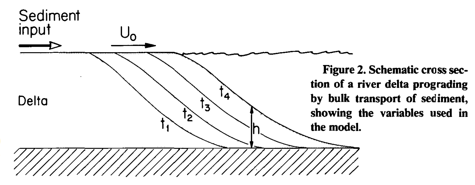
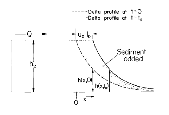
This cartoon shows the model set-up. What are the assumptions, and how does it relate to a Gilbert-type delta?

• sediment moves downslope from landward edge of delta from creep and landslides
• bulk sediment movement = diffusion
• variable slope, one process
• in the model, delta progrades at rate $u_0$, but the shape remains unchanged

print(' and '.join(picked))

Introduction and motivation

some key passages from the paper:

• "Recently, a number of papers have pointed out the prevalence of bulk-sediment movements, such as creep* and landslides, on the subaqueous portions of large deltas (and in other subaqueous environments), as opposed to the movements of individual particles stressed by Gilbert.*"
• "In subaerial environments, the geomorphic forms characteristic of sediment transport by bulk motion, and in particular by creep, differ substantially from those developed by the sliding of individual particles down a slope lying at the angle of repose (Carson and Kirkby, 1972). This difference occurs because, in landforms governed by bulk sediment movement, slope is variable and adjusts to produce the rate of transport necessary to accommodate a given supply of sediment. In contrast, in landforms governed by angle of repose, slope is fixed, and the transport rate adjusts to maintain the slope. As yet, the consequences of this difference have not been considered for subaqueous features such as deltas."

Introduction and motivation

• just a quick reminder of what was being referred to with bedload vs. suspended load

Setting-up the model: creep

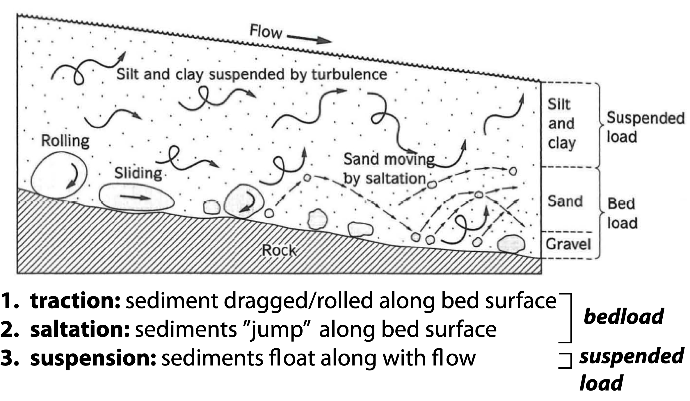
Now, let's start building the model, starting with a way to model creep. The authors introduce this equation:

$\begin{equation} \dfrac{\partial h}{\partial t} = - \dfrac{\partial S}{\partial x} \tag{equation 2} \end{equation}$

In words, what is this equation saying?

class_list,picked=pick_group(class_list)

Equation 2 is the continuity equation, and "expresses the law of conservation of mass and, neglecting compaction, should be valid for any of the bulk-transport processes we are considering."

Setting-up the model: creep

Next, the authors introduced this equation:

$\begin{equation} S = - D \dfrac{\partial h}{\partial x} \tag{equation 3} \end{equation}$

In words, what is this equation saying?

print(' and '.join(picked))

"In theoretical geomorphology, equation 3 is derived by considering the downslope bias introduced by gravity into the random motions of soil particles induced"

subaerial:	subaqeuous:
freeze-thaw, bioturbation	bioturbation, movement by waves

Setting-up the model: creep

Just like we saw in lecture yesterday, if we take the derivative of equation 3 with respect to x:

$\begin{align} S &=& - D \dfrac{\partial h}{\partial x} \tag{equation 3}\\ \dfrac{\partial S}{\partial x} &=& \dfrac{\partial}{\partial x}\Big(-D\dfrac{\partial h}{\partial x}\Big) \\ \dfrac{\partial S}{\partial x} &=& -D\dfrac{\partial^2 h}{\partial x^2} \\ \end{align}$

We can now combine with equation 2: $\begin{align} \dfrac{\partial h}{\partial t} &=& - \dfrac{\partial S}{\partial x} \tag{equation 2}\\ \dfrac{\partial h}{\partial t} &=& D\dfrac{\partial^2 h}{\partial x^2} \tag{the diffusion equation} \end{align}$

Setting-up the model: landslides

Okay, so then what about landslides? What is this equation saying, and how do we relate it to diffusion?

$\begin{equation} \tau_d = \rho g z ~ sin (\beta) \tag{equation 4} \end{equation}$

class_list,picked=pick_group(class_list)

• at low slope angles (like we encounter in deltas, $\sim$4$^{\circ}$), we can say $sin (\beta) \approx tan (\beta)$
• $\tau_d$ is the driving force for landslides
• $tan (\beta)$ = $\dfrac{\Delta h}{\Delta x}$ = $\dfrac{\partial h}{\partial x}$
• so we can say that $\tau_d \propto \dfrac{\partial h}{\partial x}$, which makes a diffusive flux
• in the term, $\rho gz$, $z$ measures depth to failure (i.e., from the surface). So, $\rho gz$ is the gravitational force from overlying slab of wet sediment that fails. This slab imparts a shear force $\tau_d$ on the failure surface

at low slope angles (like we encounter in deltas, $\sim$4$^{\circ}$), we can say $sin (\beta) \approx tan (\beta)$

Setting-up the model: creep and landslides

now we have all the parts needed: $\begin{align} S_L &=& - C \dfrac{\partial h}{\partial x} \tag{equation 7}\\ \dfrac{\partial h}{\partial t} &=& C\dfrac{\partial^2 h}{\partial x^2}\tag{equation 8}\\ \dfrac{\partial h}{\partial t} &=& (C + D)\dfrac{\partial^2 h}{\partial x^2} \tag{equation 9}\\ \dfrac{\partial h}{\partial t} &=& K\dfrac{\partial^2 h}{\partial x^2} \tag{equation 10} \end{align}$

Making the model: getting to an equation for delta morphology

To get to an analytical (h(x,t) = ...) solution for equation 10, we need to introduce some new variables. What are they? $\begin{align} \xi &=& x - u_0 t \tag{equation 11}\\ t' &=& t \tag{equation 12}\\ \end{align}$

class_list,picked=pick_group(class_list)

• t' is more conceptual - a statement that we are in a moving reference frame

• JMH notes specific to 9-18-2020 lecture:

  • We made it to this slide, with discussion lead by students
  • clear that the math is challenging - it is good to go over it!
  • made it through 11 slides / sub-slides in 50 minutes, still have 5 to go.
  • one, however, is quite open-ended $\rightarrow$ discussion of data-model comparisons.

"An analytic solution of equation 10 for steady progradation can be obtained in a coordinate system moving with the landward edge of the delta front"

Making the model: getting to an equation for delta morphology

How are these new variables used in these new equalities? $\begin{align} \dfrac{\partial h}{\partial x}&=&\dfrac{\partial h}{\partial \xi} \tag{equation 13}\\ \dfrac{\partial h}{\partial t}&=&\dfrac{\partial h}{\partial t'} - u_0\dfrac{\partial h}{\partial \xi} \tag{equation 14}\\ \dfrac{\partial h}{\partial t'} &=& 0 \tag{equation 16}\\ \end{align}$

class_list,picked=pick_group(class_list)

Making the model: getting to an equation for delta morphology

How are these new variables used in these new equalities? $\begin{align} \dfrac{\partial h}{\partial x}&=&\dfrac{\partial h}{\partial \xi} \tag{equation 13}\\ \dfrac{\partial h}{\partial t}&=&\dfrac{\partial h}{\partial t'} - u_0\dfrac{\partial h}{\partial \xi} \tag{equation 14}\\ \dfrac{\partial h}{\partial t'} &=& 0 \tag{equation 16}\\ \dfrac{\partial h}{\partial t'} - u_0 \dfrac{\partial h}{\partial \xi} &=& K \dfrac{\partial^2 h}{\partial \xi^2} \tag{equation 15}\\ 0 &=& \dfrac{\partial^2 h}{\partial \xi^2} + \dfrac{u_0}{K} \dfrac{\partial h}{\partial \xi} \tag{equation 17} \end{align}$

Making the model: getting to an equation for delta morphology

because we are ONLY differentiating with respect to $\xi$, we can express equation 17 as an ordinary differential equation ($\partial \rightarrow d$): $\begin{equation} 0 = \dfrac{d^2 h}{d \xi^2} + \dfrac{u_0}{K} \dfrac{d h}{d \xi} \tag{equation 17}\\ \end{equation}$ this equation has the general form:

$0 = y'' + Cy'$

Using the model: comparing to real world

combined with the restraint that $h = h_0$ at the top of the delta, we now have an equation that predicts how the height of the delta changes with increasing distance into the basin:

$\begin{equation} h(x,t) = h_0 e^{-\frac{u_0}{K} (x - u_0 t)} \end{equation}$

but to better facilitate data-model comparisons, it is helpful to consider the delta front slope:

$\begin{equation} \dfrac{\partial h}{\partial x} = \dfrac{-u_0 h}{K}~~~~\rightarrow~~~~~ K = \dfrac{-u_0 h}{(\partial h/\partial x)} \end{equation}$

Why is the above equation useful, and what can be done with it?

• with bathmyetry data and progradation estimates, you can estimate K
• use K to predict full delta profile

class_list,picked=pick_group(class_list)

Using the model: comparing to real world

However, constraining $u_0$ for real deltas is rather tricky (why?). By constrast, constraining the time-averaged volumetric sediment ($Q$) to a delta is more tractable. If we consider a span of time $t_0$, the volume of sediment added is given by the shaded region in the figure below. This volume can be calculated as:

$\begin{equation} Qt_0 = h_0u_0t_0 ~~~~\rightarrow~~~~~ u_0 = \dfrac{Q}{h_0} \end{equation}$
Why are the above equalities correct? (hint: no complicated integral calculus is required)

print(' and '.join(picked))

Using the model: comparing to real world

So how did this model compare to real data? (I can pull up specific figures on the PDF for discussion)

class_list,picked=pick_group(class_list)

Assignment 1.1: exploring diffusive deltas

This weeks assignment will give you some experience with coding and plotting and further explore the concepts and ideas laid out in Kenyon and Turcotte (1985):

• You are not excluded from working with other groups.
• Each person will submit their own copy of the assignment
• Assignment due date: January 27, 2023 by 1:30PM, via uploaded PDF to Brightspace