Lecture 8-10: Time in Stratigraphic Sequences
- Gross vs. net fluxes
- an illustrative example
- diastems and hiatuses
- how to build a rock record
- The concept of correlation
- Chronostratigraphy (Wheeler diagrams)
- Time in the rock record
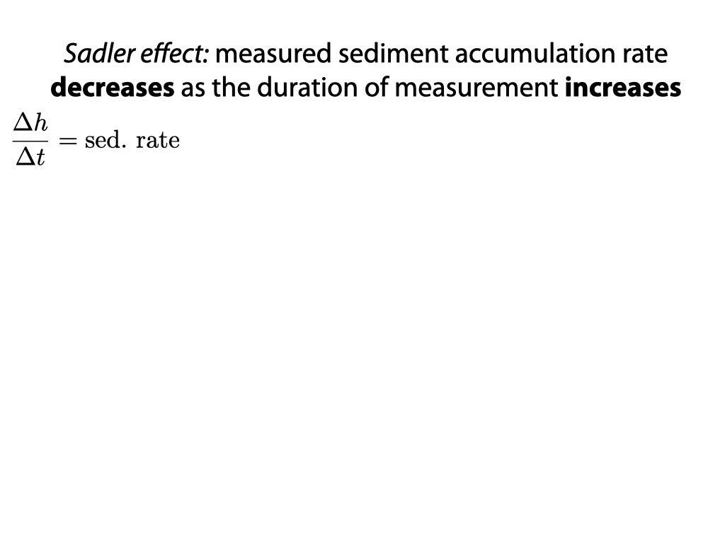
- Sadler effect
We acknowledge and respect the lək̓ʷəŋən peoples on whose traditional territory the university stands and the Songhees, Esquimalt and W̱SÁNEĆ peoples whose historical relationships with the land continue to this day.
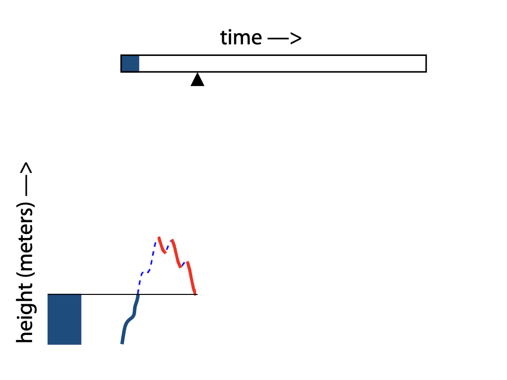
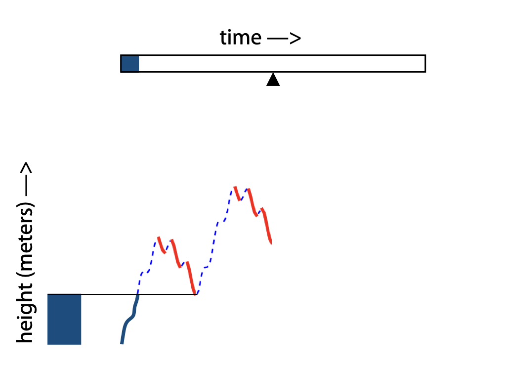
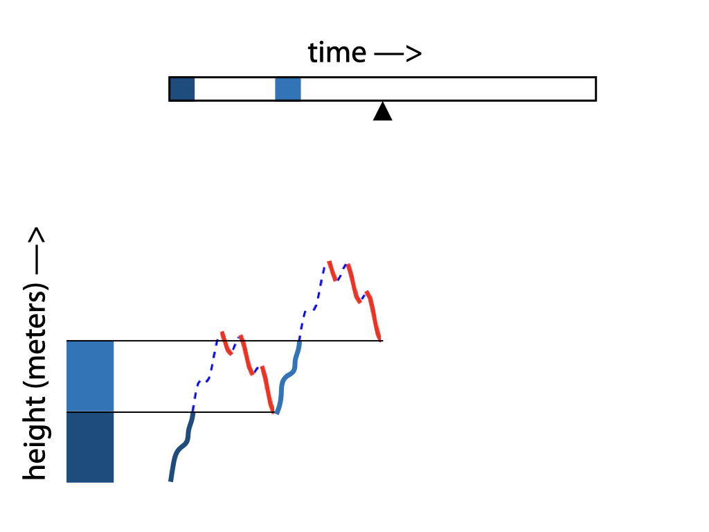
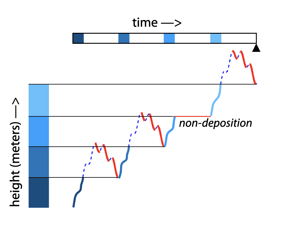
Gross vs. Net fluxes
Gross and net sedimentation
Gross and net sedimentation
Gross and net sedimentation
Gross and net sedimentation
Gross and net sedimentation
Gross and net sedimentation
Gross and net sedimentation
Gross and net sedimentation
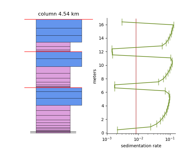
net sedimentary record is full of gaps: both erosive surfaces and hiatuses.
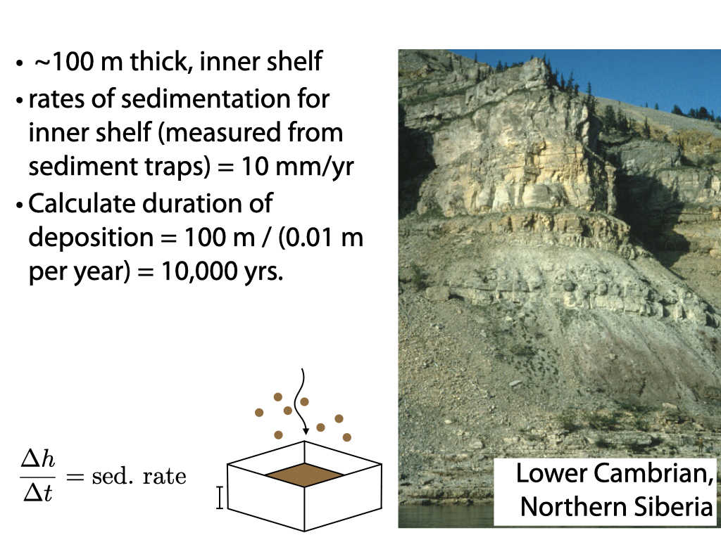
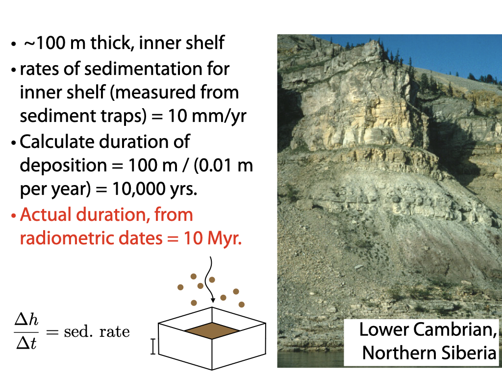
How much time is represented by sedimentary rock?
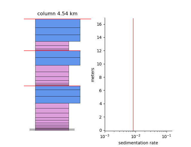
How to build the net rock record
In [4]:
import csv
import numpy as np
from matplotlib import pyplot as plt
import seaborn as sns
sns.set_context('talk')
%matplotlib inline

#empty lists for data
model_topo=[]

#open the data file
with open("../Assignments/Assignment_1/Assignment_1p3/data/model_results.csv","r") as fid:
    data = csv.reader(fid, delimiter=",")

    #reads the data in line-by-line
    for row in data:
        model_topo.append([float(r) for r in row[1:]])

#convert to list of numpy arrays
model_topo=[np.array(t) for t in model_topo]

#define as change from inital conditions
model_topo=[t-model_topo[0] for t in model_topo]
How to build the net rock record
In [5]:
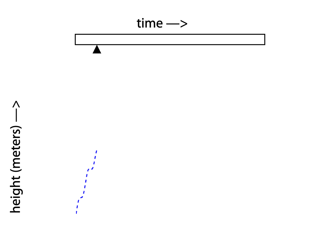
#pull topographic evolution from one spot in the basin
section=[t[454] for t in model_topo]

plt.plot(section,'-',color='r')
plt.plot(np.arange(len(section))[0::4],section[0::4],'.',markersize=5,color='k')

plt.gca().set_xticks([])
plt.gca().set_xlabel(r'time $\rightarrow$')
plt.gca().set_ylabel('height (meters)')
plt.gca().xaxis.set_label_position('top')

How to build the net rock record
In [3]:
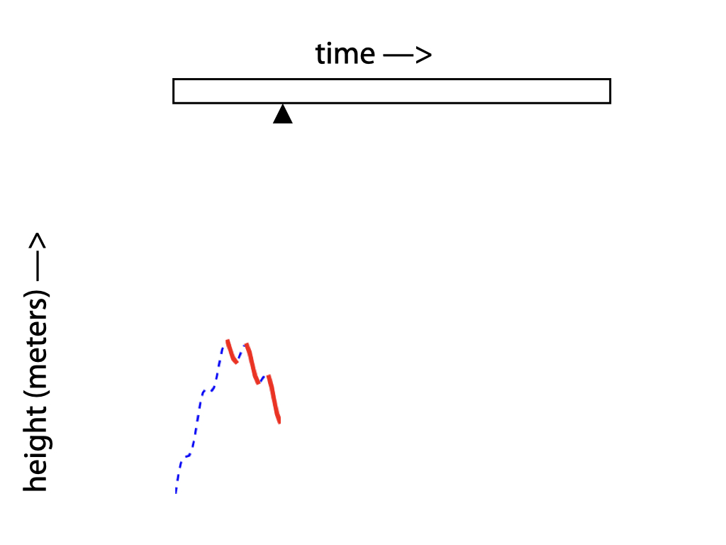
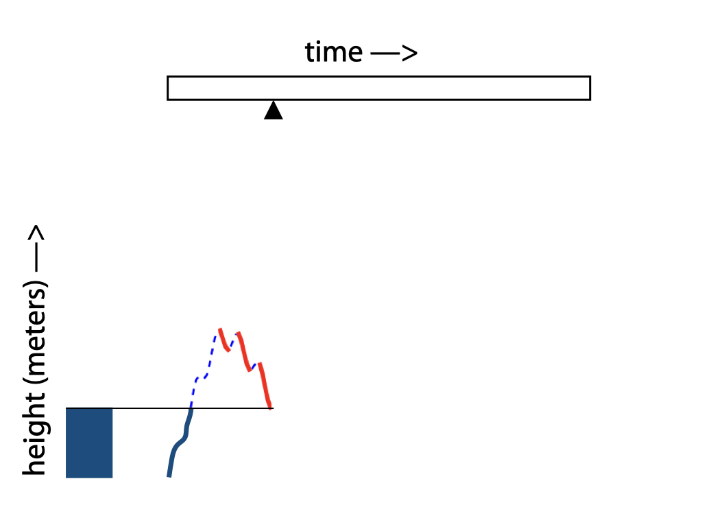
net=np.flipud(section) #flip this stratigraphy upside down to examine youngest to oldest
for i,s in enumerate(net): #count through time slices starting at the youngest
    if i!=len(net)-1: #if we're not at the end
        #look "down section" - was this layer eroded?
        # --> if height had decreased, then yes
        if s<net[i+1]: #s is height of current timeslice, net[i+1] is heigh of previous timeslice
            net[i+1]=s #create new record of net sedimentation
#make stratigraphy younging upwards again
net=np.flipud(net)
plt.plot(net,color='b')
plt.fill_between(np.arange(len(section)),section,net,color='r',alpha=0.25)
plt.gca().set_xticks([])
plt.gca().set_xlabel(r'time $\rightarrow$')
plt.gca().set_ylabel('height (meters)')
plt.gca().xaxis.set_label_position('top')

How to build the net rock record
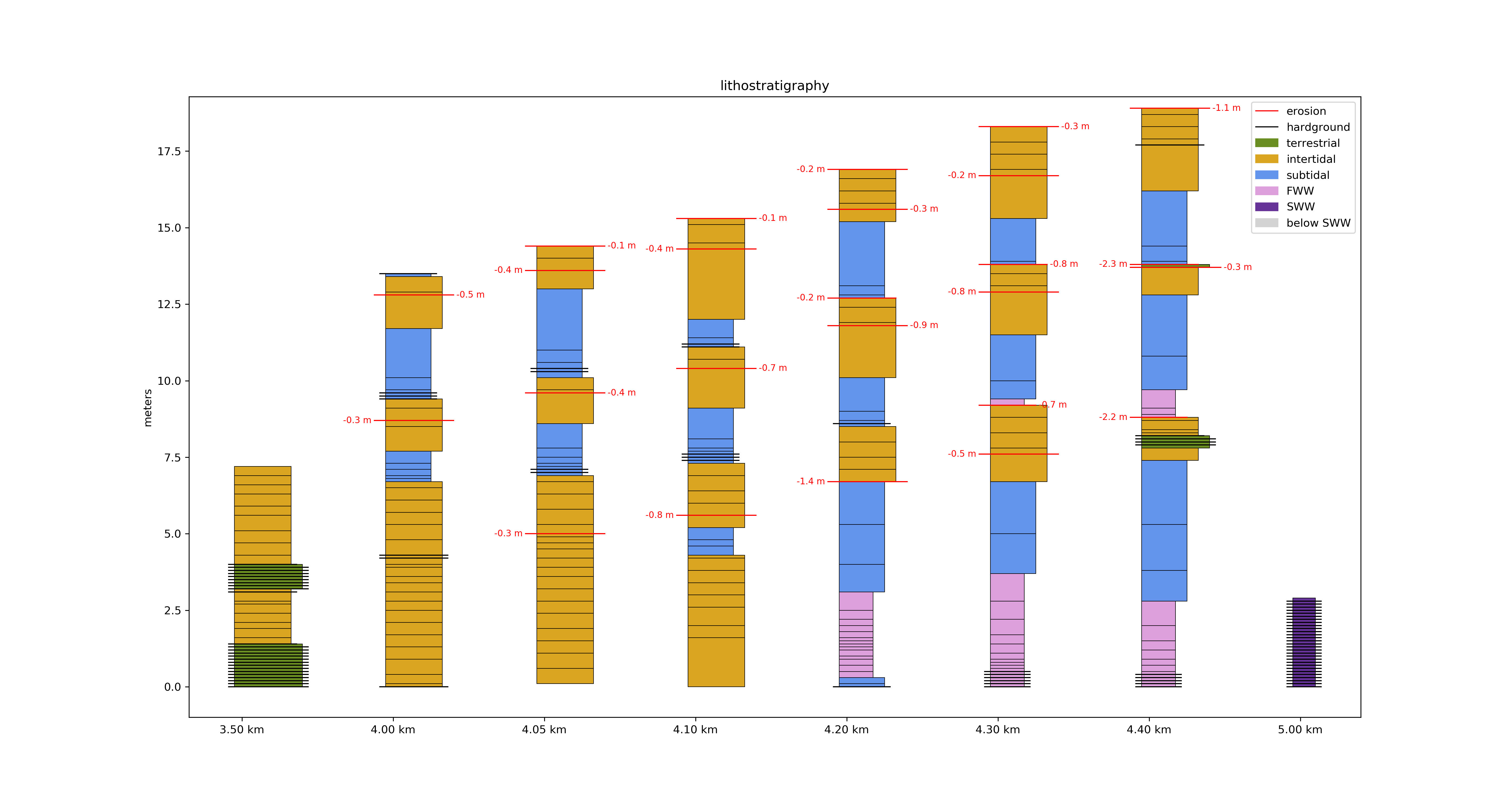
Chronostratigraphy and Wheeler Diagrams
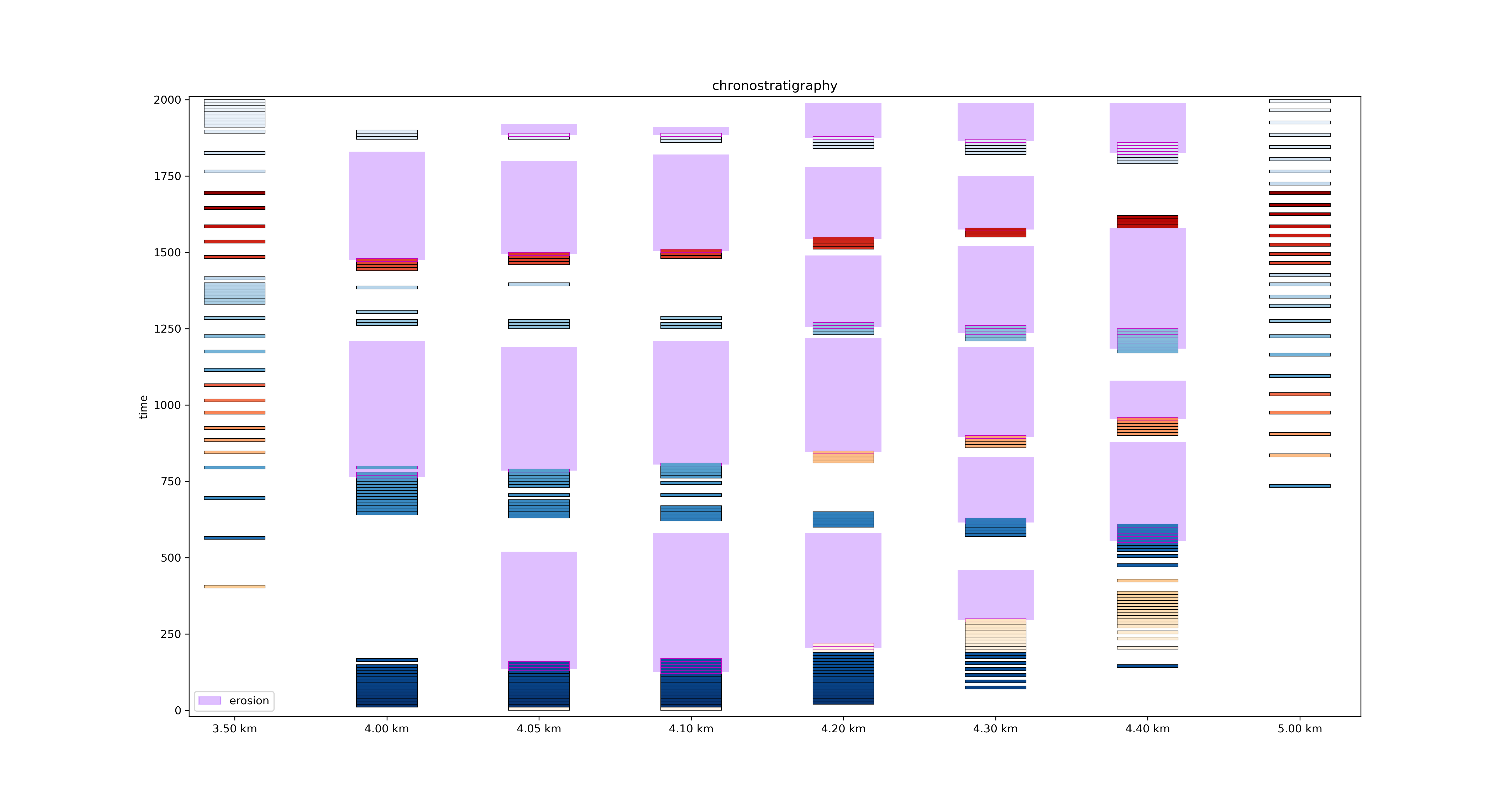
Chronostratigraphy and Wheeler Diagrams

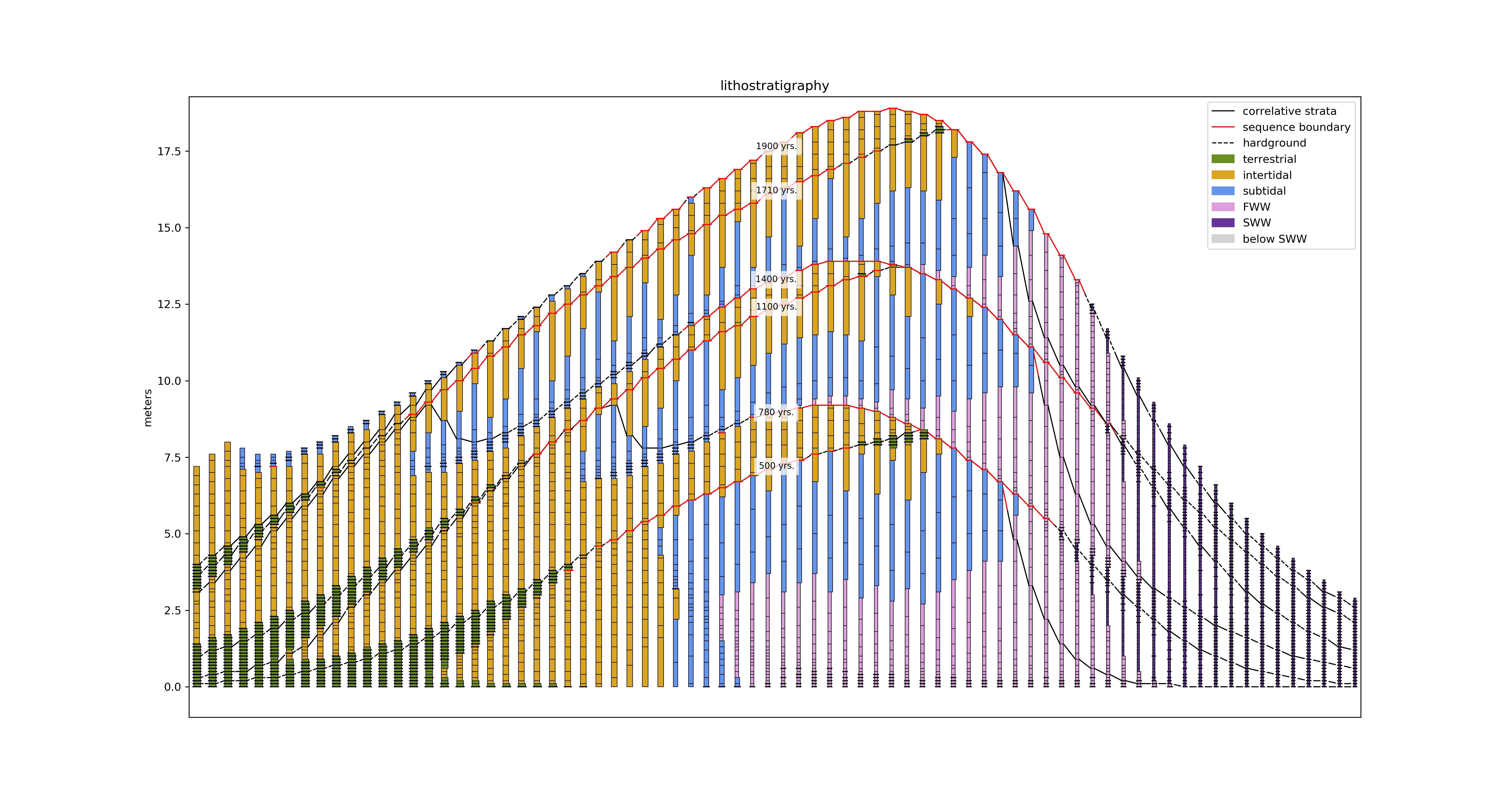
Correlating in lithostratigraphic space
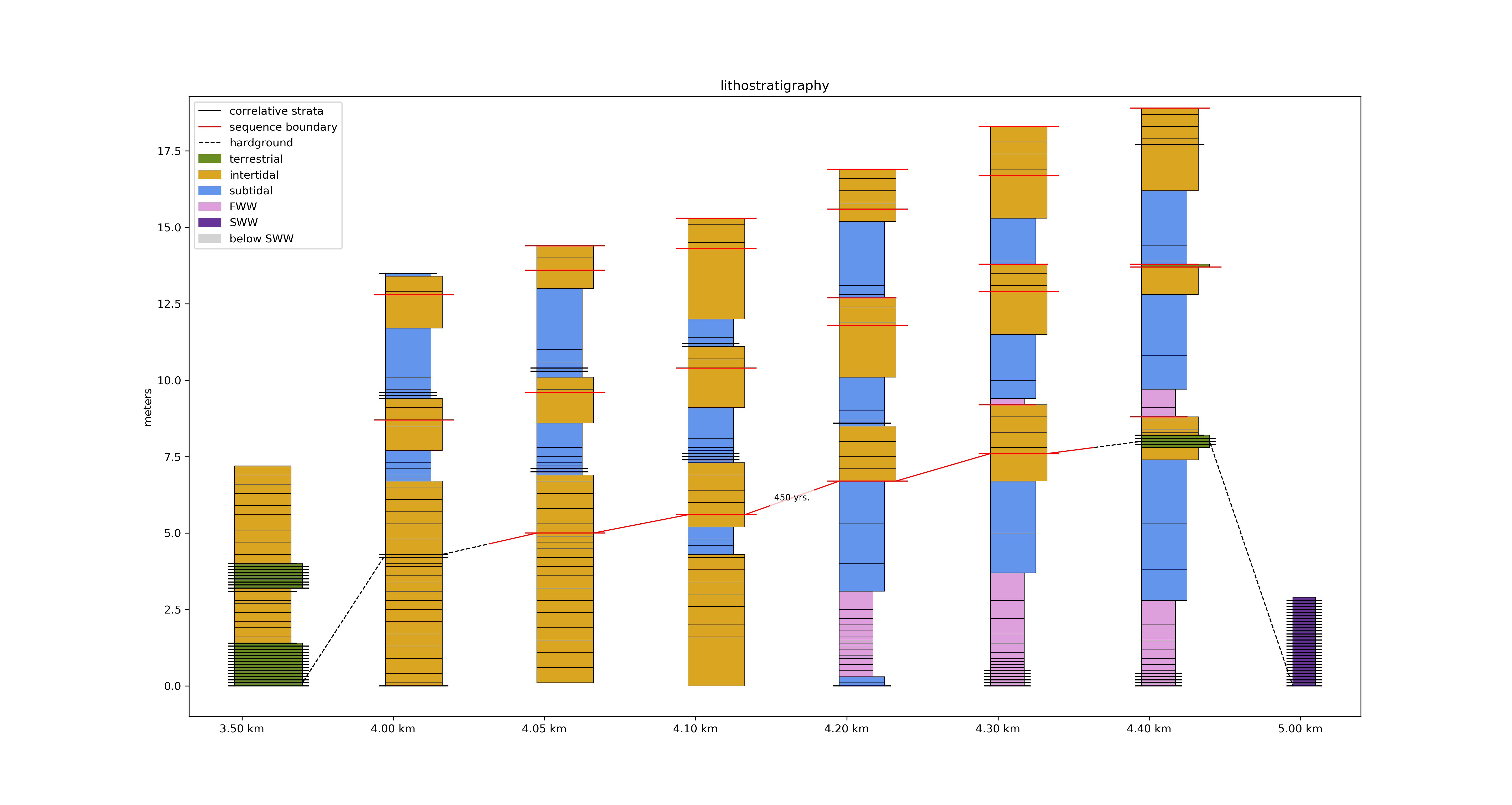
Correlating in lithostratigraphic space

Correlating works best with many sections!
Correlating works best with many sections!
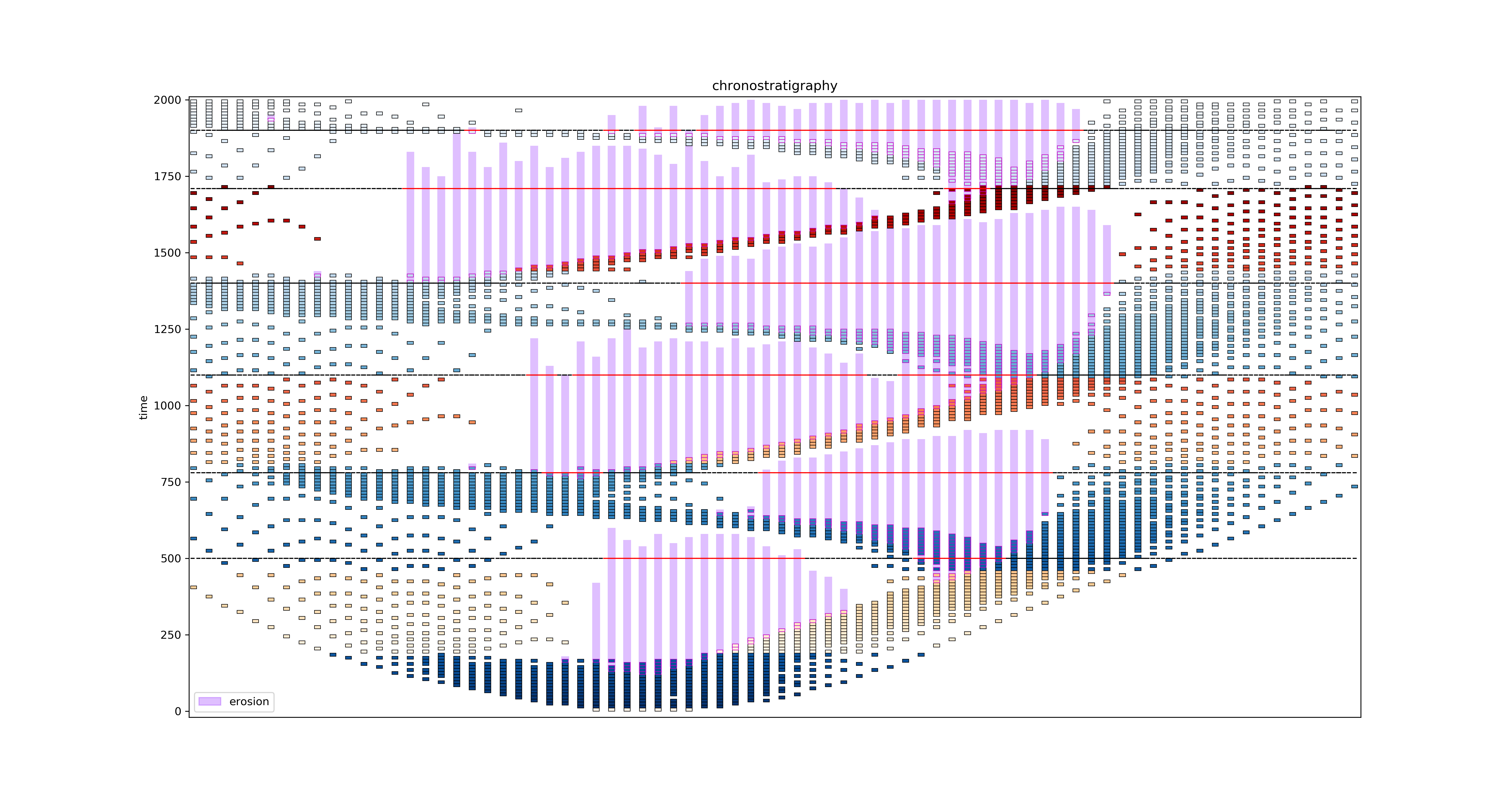
Time in the rock record
Time in the rock record
Time in the rock record
Time in the rock record

Time in the rock record
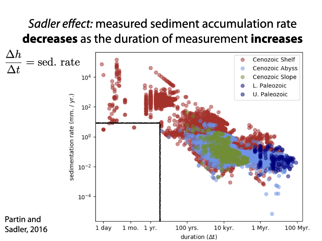
Why is this happening?
Time in our rock record
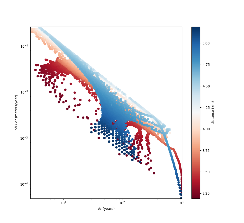
Why is this happening?