Lectures 11-12: Cycles
- Quantitative correlation
- An example from our model
- Enter cyclostratigraphy
- How to identify a cycle
- Fourier Transforms
We acknowledge and respect the lək̓ʷəŋən peoples on whose traditional territory the university stands and the Songhees, Esquimalt and W̱SÁNEĆ peoples whose historical relationships with the land continue to this day.
Brief return to Wheeler diagrams
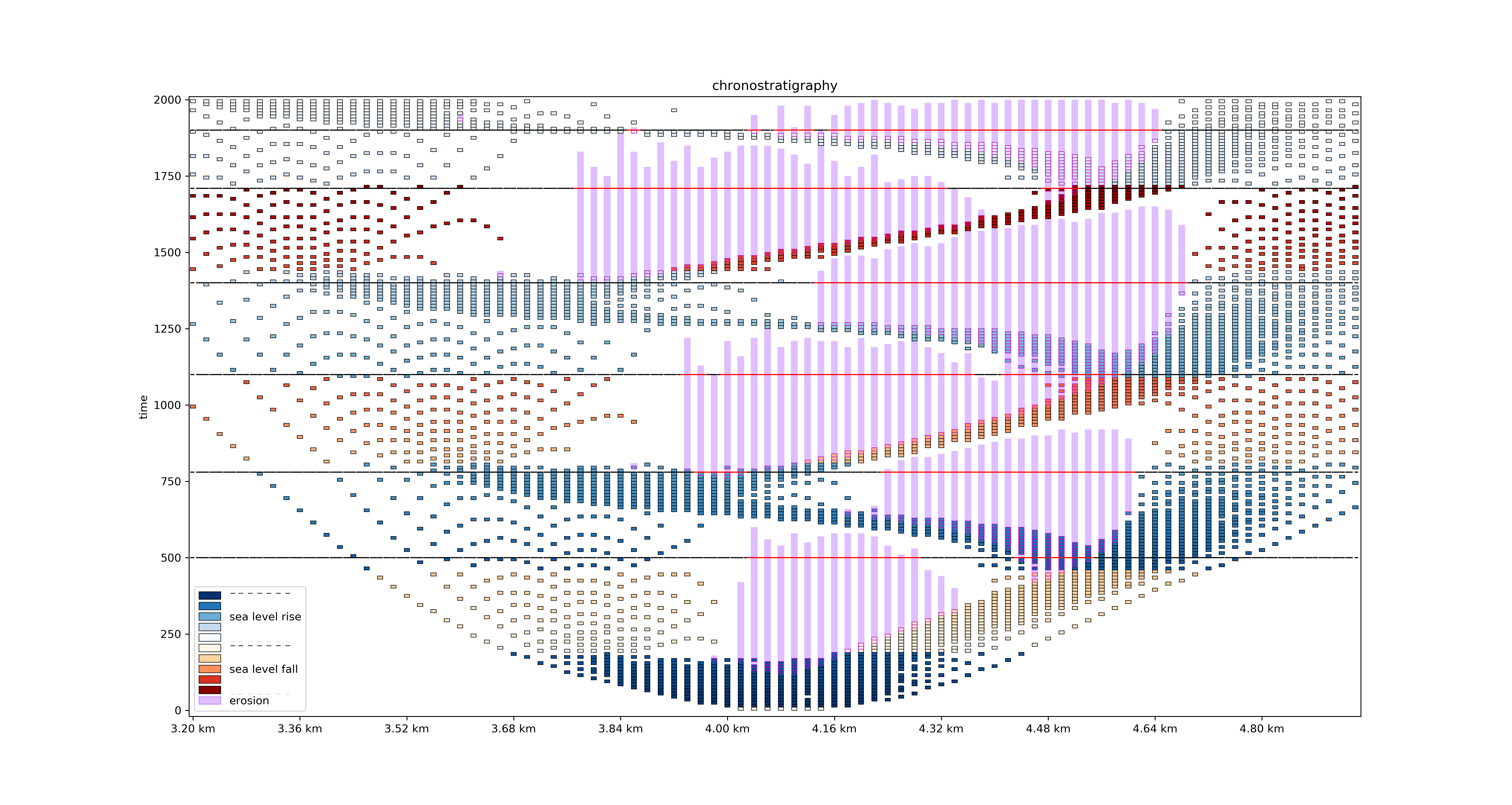
Brief return to Wheeler diagrams
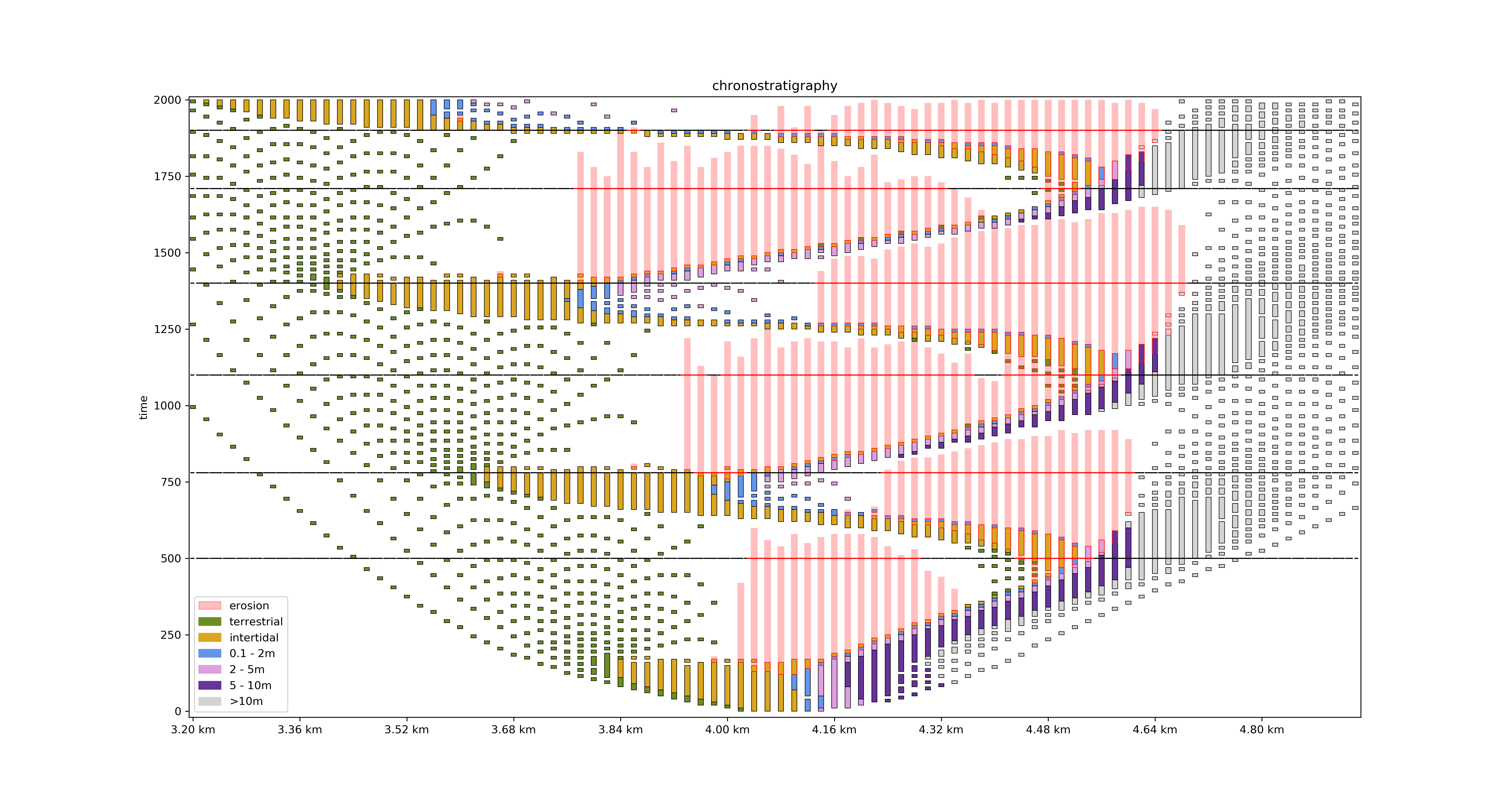
Brief return to Wheeler diagrams
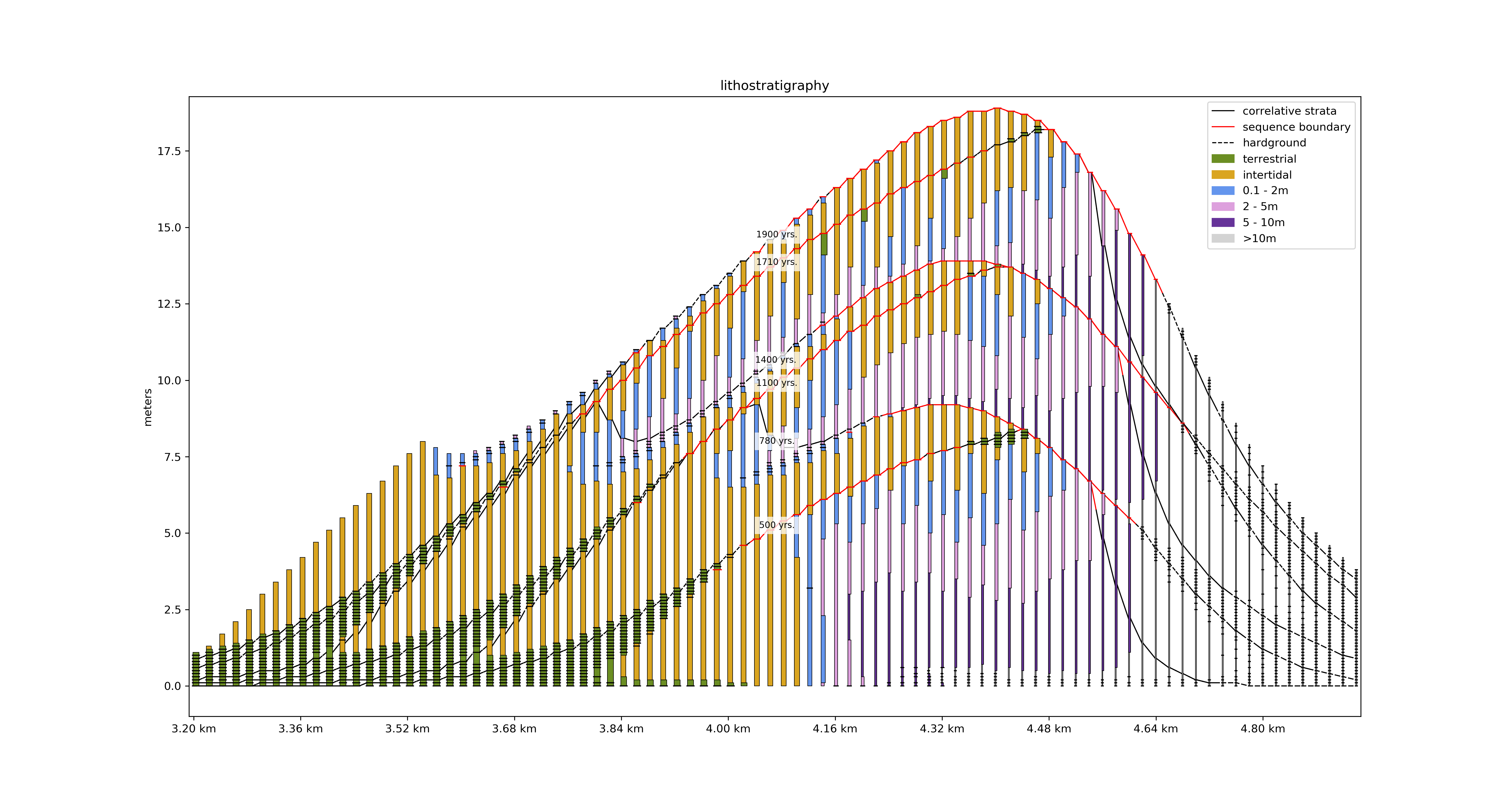
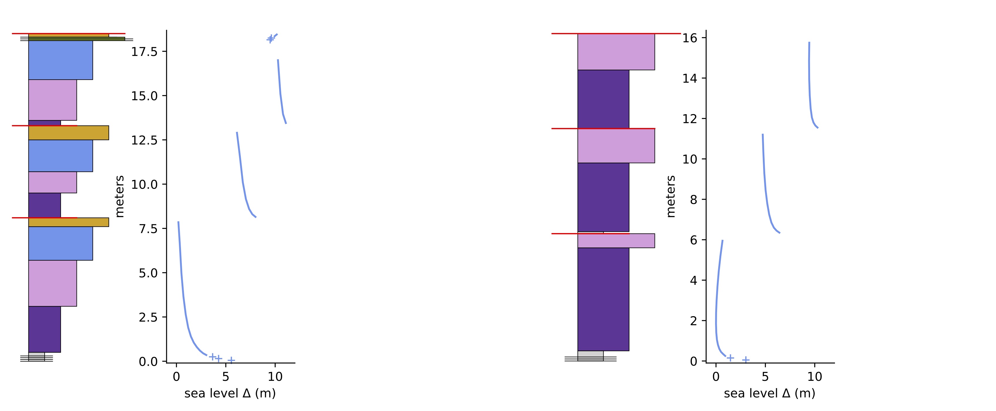
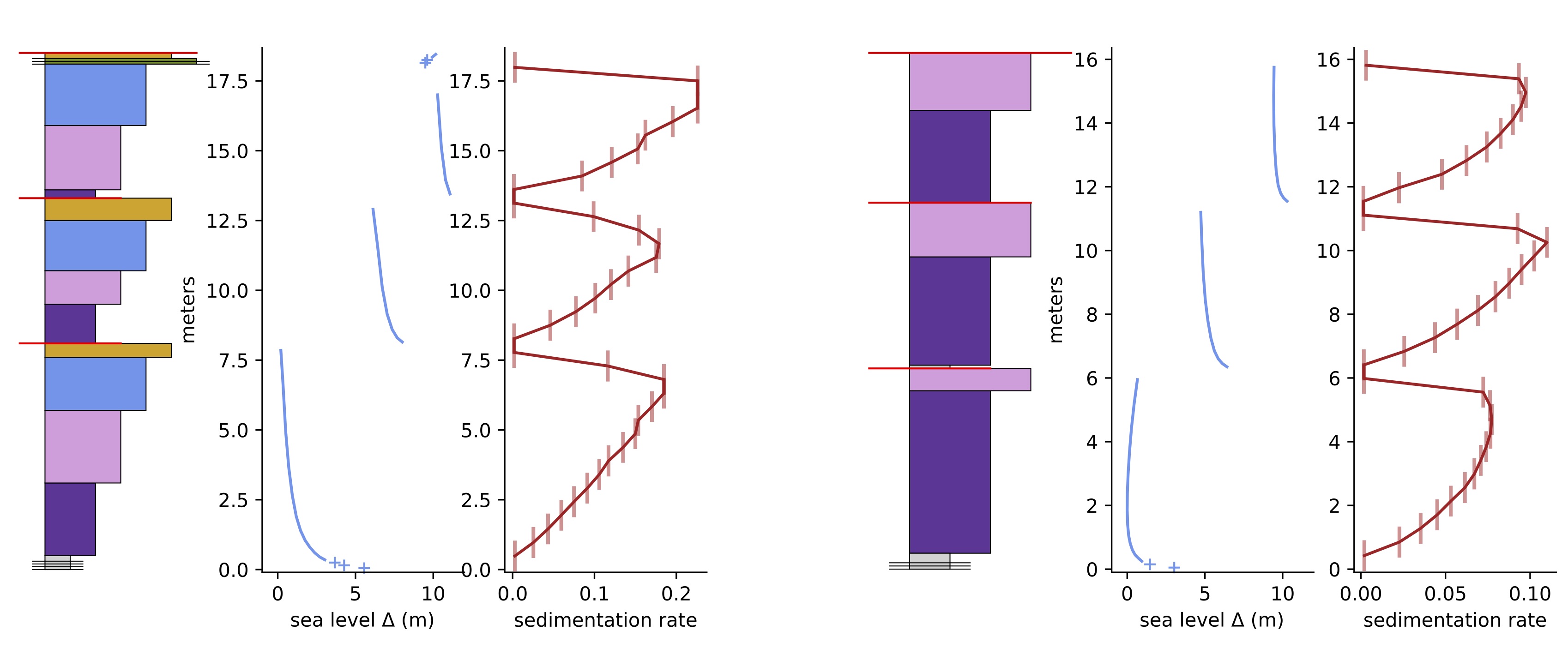
Correlating sequences: an example from our model

Correlating sequences: an example from our model
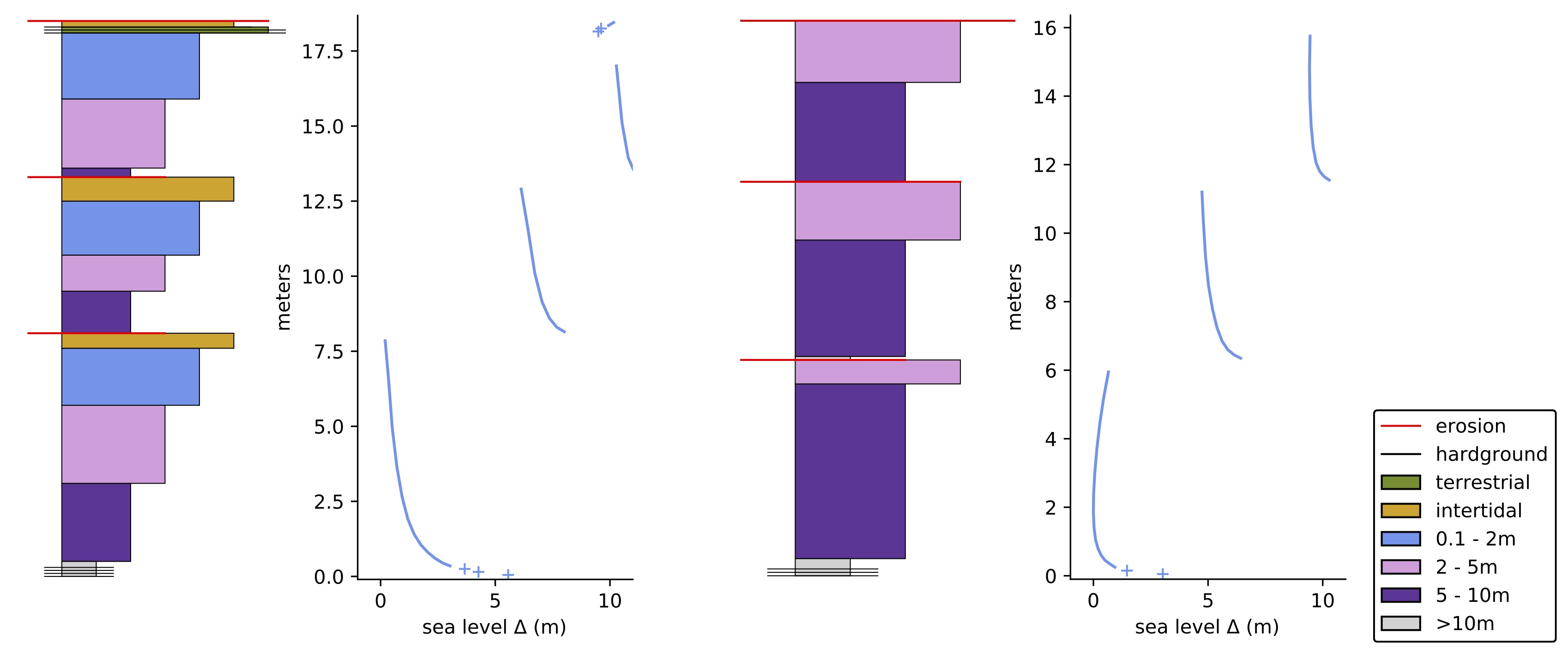
Correlating sequences: an example from our model
Correlating sequences: an example from our model
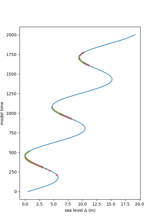
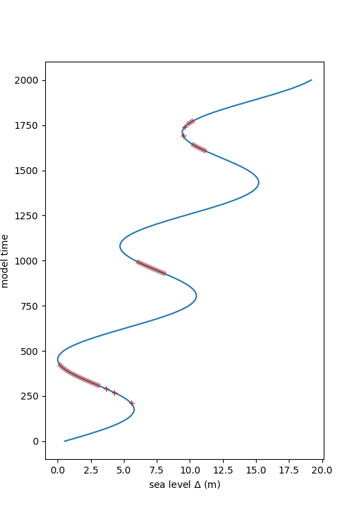
Why do the sea-level cycles look funny?
Why do the sea-level cycles look funny?
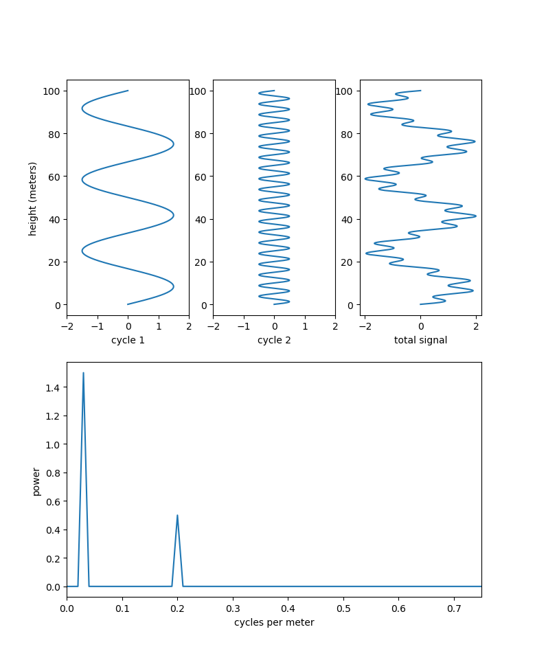
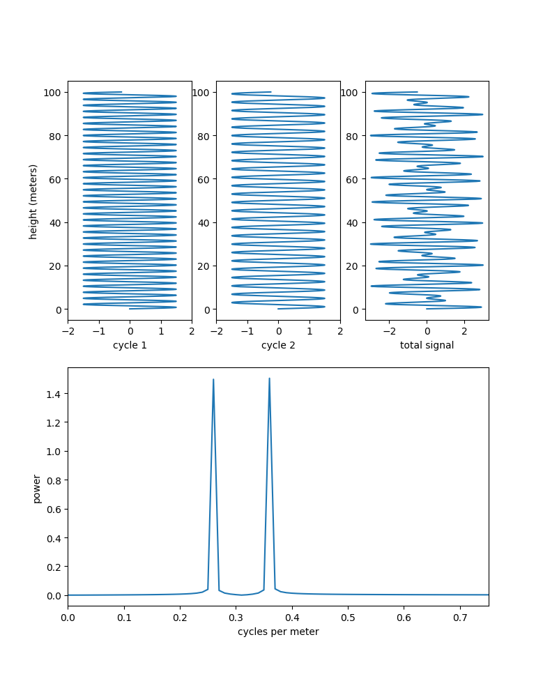
Correlating sequences
- an amazing key would be detecting this sea level signal
- how could this be done?
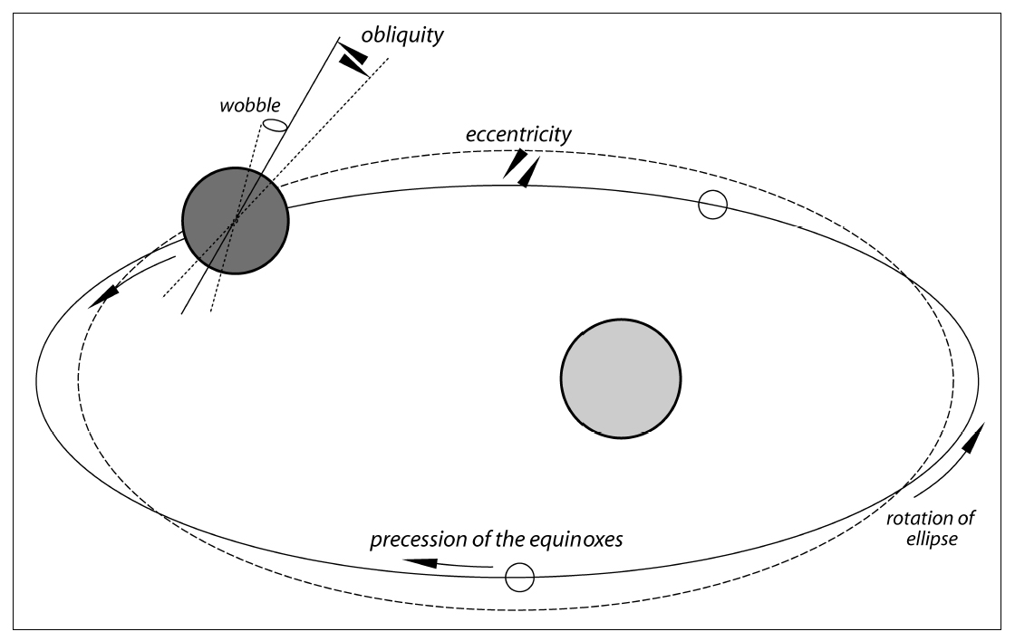
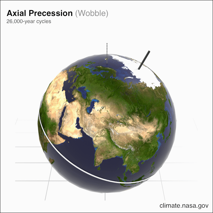
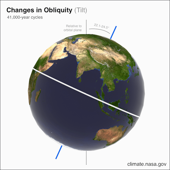
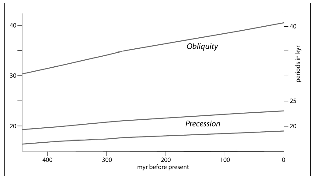
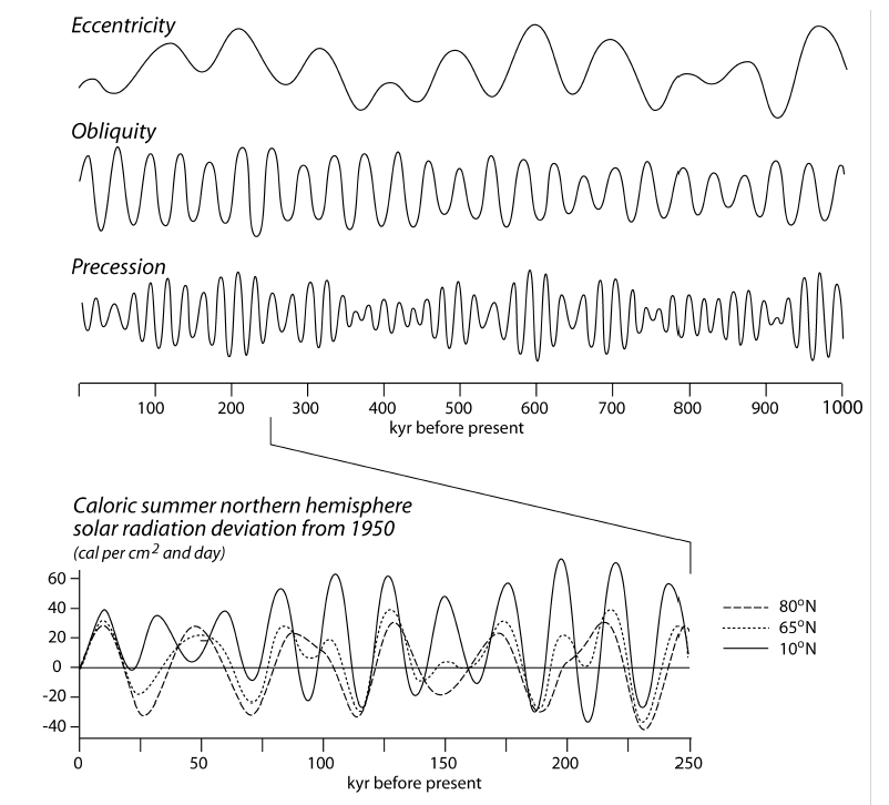
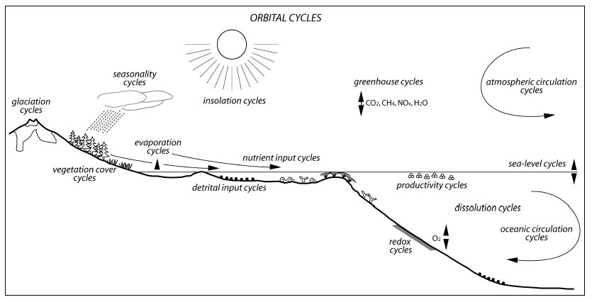
Cyclostratigraphy
- Cyclostratigraphy is a sub-discipline of stratigraphy that seeks to identify, characterize and interpret cyclic variations in the stratigraphic record
- identify cycles $\rightarrow$ interpret timing of cycles $\rightarrow$ age models and correlations
- fundamentally, it is about explaining the processes behind a record
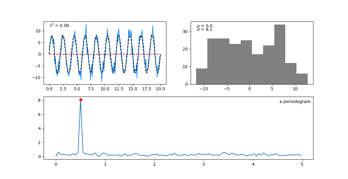
Identifying cycles
In [5]:
t = 20 # total time series
N=200 # sample spacing
x = np.linspace(0.0, t, N) #noise amplitude
a=2
noise=np.random.normal(0,a,N) #total signal
y=x+noise # plot_data_res(x,y)
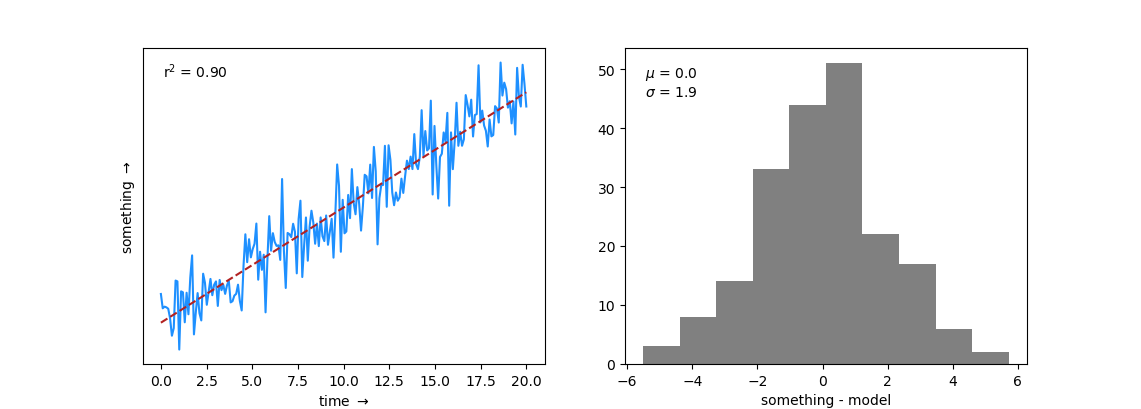
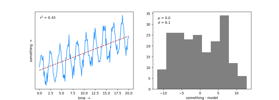
Identifying cycles
In [10]:
#add a sine wave
y=y+8*np.sin(0.5*2*np.pi*x)

#plot_data_res(x,y)
Identifying cycles
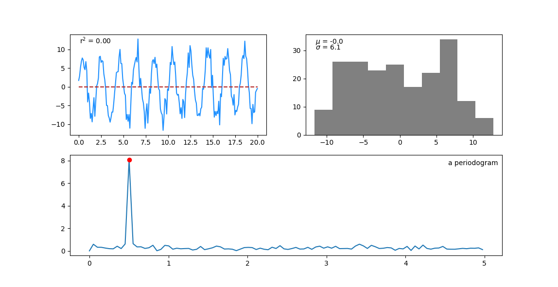
In [6]:
#remove the linear rise
y=signal.detrend(y)
#define sampling interval for frequency axis
dt=np.round(np.diff(x),10)[0]
#perform Fast Fourier transform
yf = fft(y)
xf = np.linspace(0.0, 1.0/(2.0*dt), N//2)
#plot results
# axes,max_power,freq=plot_data_res_fft(x,y,yf,xf)
Identifying cycles
In [8]:
#create and plot the recovered sinusoid
amp=max_power
ang_freq=freq * 2*np.pi
phase=0 * np.pi/180
cycle=amp*np.sin(ang_freq*x + phase)
#axes,max_power,freq=plot_data_res_fft(x,y,yf,xf)
#axes[0].plot(x,cycle,'k--')
Identifying cycles
In [18]:
##recalculate residuals
#axes=plot_data_res_fft(x,y-cycle,yf,xf)
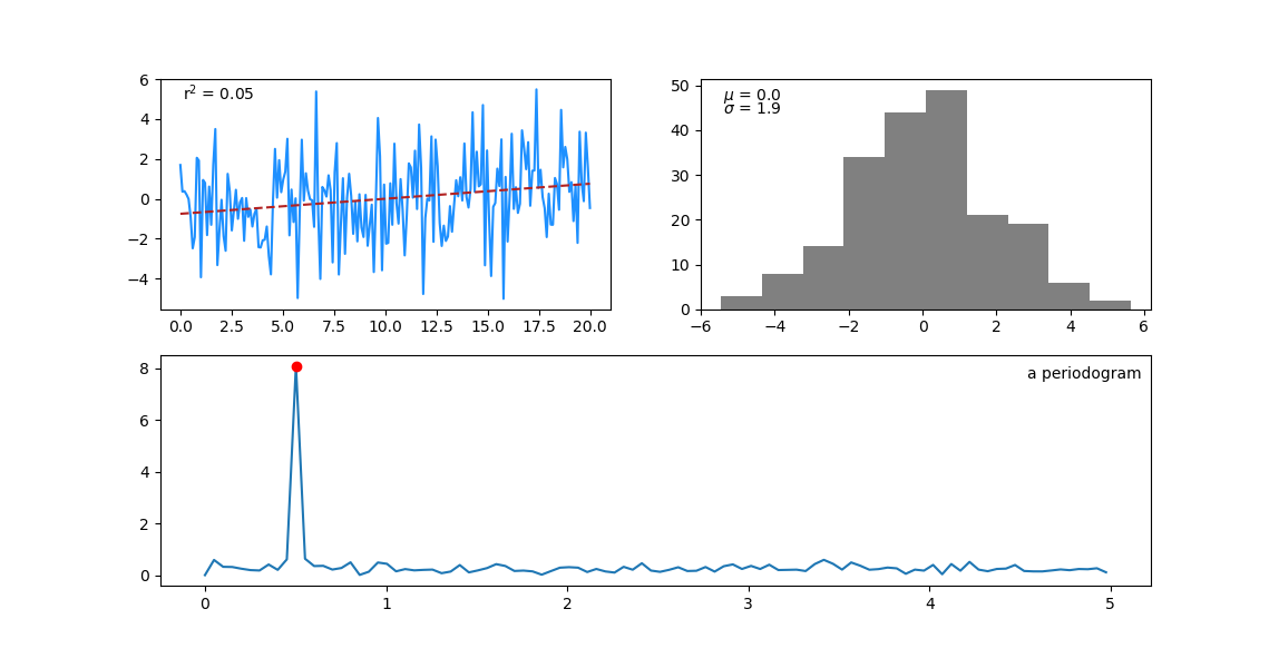
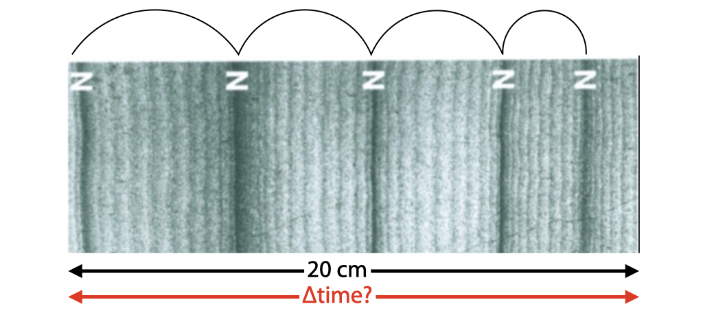
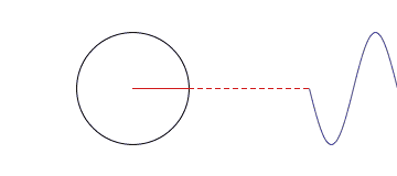
quickly we cannot rely on our eyes ...
quickly we cannot rely on our eyes ...
quickly we cannot rely on our eyes ...
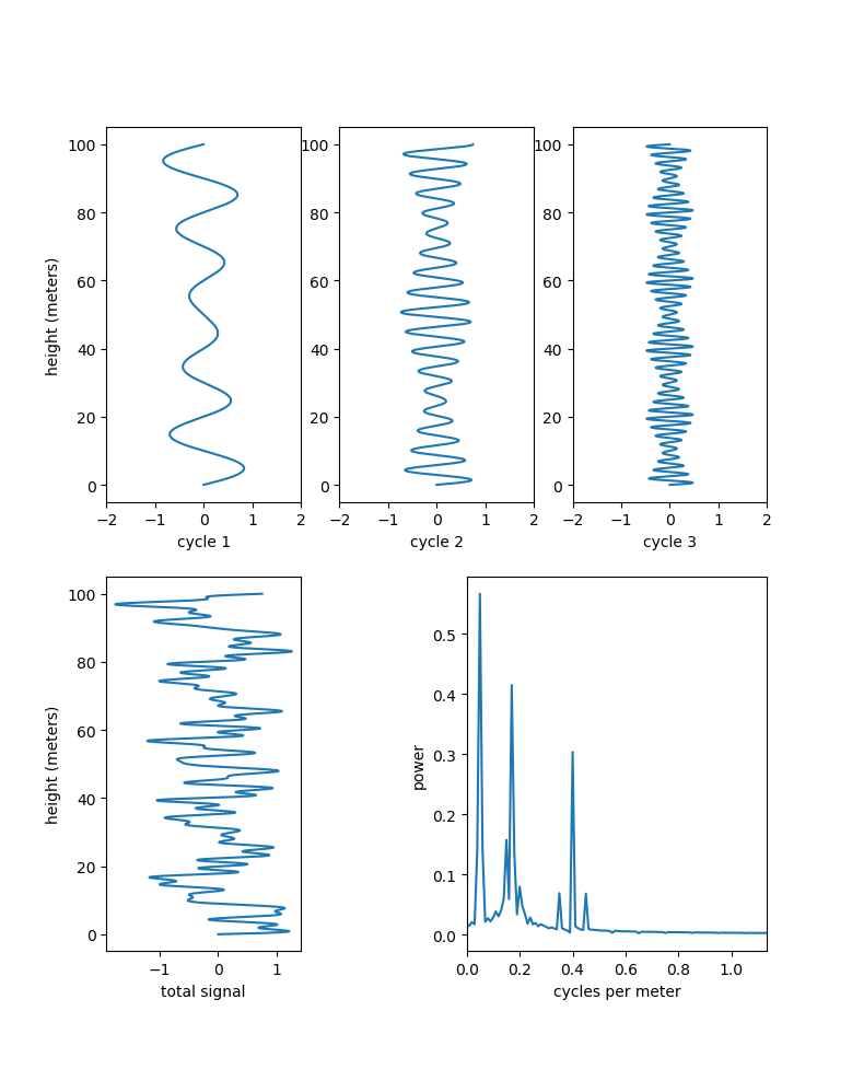
quickly we cannot rely on our eyes ...
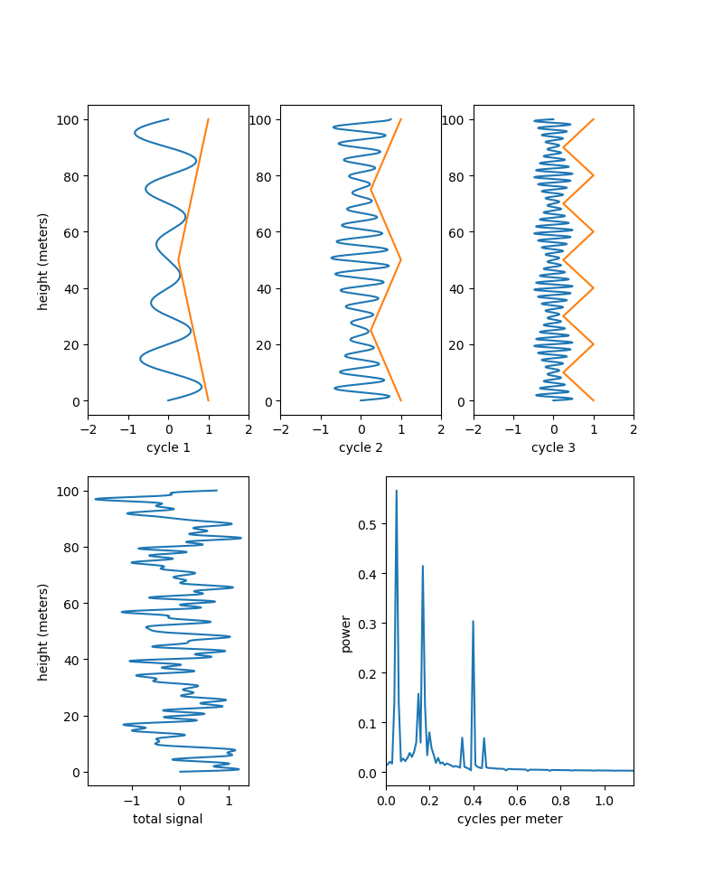
(Draw cycles in sediments)
Information can be described as an infinite series of sin and cos waves of differing frequencies and magnitudes.
In [6]:
plt.figure(figsize=(25,5))
plt.subplot(1,2,1)
xt = np.linspace(0,4,1000)
y = (np.cos(xt*3*2*np.pi)+1)/2
plt.plot(xt,y,lw=2)
plt.gca().set_title('3 beats/second',y=1.1)
plt.gca().set_xlabel('Time (s)')
plt.subplot(1,2,2, polar=True)
_=plt.gca().set_yticklabels([])

In [7]:
plt.figure(figsize=(25,5))
plt.subplot(1,2,1)
xt = np.linspace(0,4,1000)
y = (np.cos(xt*3*2*np.pi)+1)/2
plt.plot(xt,y,lw=2)
plt.gca().set_title('3 beats/second',y=1.1)
plt.gca().set_xlabel('Time (s)')
plt.subplot(1,2,2, polar=True)
plt.plot(xt*.5*2*np.pi,y,alpha=1,lw=2)
plt.gca().set_yticklabels([])
_=plt.gca().set_title('0.5 cycles/second',y=1.1)

Some set up to cycle through different frequencies:
In [10]:
%%capture
import time
import pylab as pl
from IPython import display
xt = np.linspace(0,4,1000)
y = (np.cos(xt*3*2*np.pi)+1)/2
y = (np.cos(xt*3*2*np.pi)+1)/4+(np.cos(xt*2*2*np.pi)+1)/4
plt.gca().set_title('3 beats/second',y=1.1)
plt.gca().set_xlabel('Time (s)')
Wrapping the signal (left) around the unit circle (right) at different frequencies:
In [ ]:
for i in np.linspace(.1,6,100):
    fig=plt.figure(figsize=(15,5))
    plt.subplot(1,2,1)
    plt.plot(xt,y,lw=2)
    plt.subplot(1,2,2, polar=True)
    display.clear_output(wait=True)
    plt.plot(xt*i*2*np.pi,y,alpha=1,lw=2)
    plt.gca().set_yticklabels([])
    _=plt.gca().set_title(f'{i:.2f} cycles/second',y=1.1)
    display.display(pl.gcf())
    time.sleep(.25)
In [12]:
plt.figure(figsize=(25,5))
plt.subplot(1,2,1)
xt = np.linspace(0,4,1000)
y = (np.cos(xt*3*2*np.pi)+1)/2
plt.plot(xt,y,lw=2)
plt.gca().set_title('3 beats/second',y=1.1)
plt.gca().set_xlabel('Time (s)')
plt.subplot(1,2,2, polar=True)
plt.plot(xt*.5*2*np.pi,y,alpha=0)
plt.plot(xt*5*2*np.pi,y)
plt.gca().set_yticklabels([])
plt.gca().set_title('5 cycles/second',y=1.1)
Out[12]:
Text(0.5, 1.1, '5 cycles/second')

In [13]:
plt.figure(figsize=(25,5))
plt.subplot(1,2,1)
xt = np.linspace(0,4,1000)
y = (np.cos(xt*3*2*np.pi)+1)/2
plt.plot(xt,y,lw=2)
plt.gca().set_title('3 beats/second',y=1.1)
plt.gca().set_xlabel('Time (s)')
plt.subplot(1,2,2, polar=True)
plt.plot(xt*.5*2*np.pi,y,alpha=1) #add back
plt.plot(xt*5*2*np.pi,y,alpha=0)
plt.plot(xt*3*2*np.pi,y)
plt.gca().set_yticklabels([])
plt.gca().set_title('3 cycles/second',y=1.1)
Out[13]:
Text(0.5, 1.1, '3 cycles/second')

Euler's formula $$ e^{ix} = cos x + i~sin x $$
In [20]:
plt.figure(figsize=(25,5))
plt.subplot(1,2,1)
xt = np.linspace(0,4,1000)
y = -1 + (np.cos(xt*3*2*np.pi)+1)/4+(np.cos(xt*2*2*np.pi)+1)/4
plt.plot(xt,y)
plt.gca().set_title('3 beats/second + 2 beats/second',y=1.1)
plt.gca().set_xlabel('Time (s)')
plt.subplot(1,2,2, polar=True)
# plt.polar(xt*.5*2*np.pi,y,label='0.5 c/s')
# plt.polar(xt*2*2*np.pi,y,label='2 c/s')
plt.plot(xt*.01*2*np.pi,y,label='3 c/s')
# plt.gca().set_yticklabels([])
# plt.legend(loc='lower right',fontsize=10,bbox_to_anchor=(1.3, -.1))
plt.gca().set_title('3 cycles/second',y=1.1)
Out[20]:
Text(0.5, 1.1, '3 cycles/second')

In [17]:
plt.figure(figsize=(25, 5))
plt.subplot(1, 2, 1)
xt = np.linspace(0, 4, 1000)
y = (np.cos(xt * 3 * 2 * np.pi) + 1) / 4 + (np.cos(xt * 2 * 2 * np.pi) + 1) / 4 - .5
complex_y = y * np.exp(-2 * np.pi * 1j * 3 * xt) #using imaginary j  and exp to convert to polar
plt.plot(complex_y.real, complex_y.imag)
plt.gca().set_aspect(1); plt.gca().set_title("3 cycles/second"); plt.subplot(1, 2, 2)
x_COM = []
freqs = np.linspace(0.1, 10, 1000)
# freqs = np.arange(0,1000-1)
for i in freqs:
    complex_y = y * np.exp(-2 * np.pi * 1j * i * xt)
    x_COM.append((np.sum(complex_y.real)**2+np.sum(complex_y.imag)**2)**(1/2))

plt.plot(freqs, x_COM,alpha=1,zorder=2); _ = plt.gca().set_xticks(range(0, 11)); plt.gca().set_ylabel("'sum'"); plt.gca().set_xlabel("frequency", y=1.1)
plt.gca().set_xlim([0,10])
Out[17]:
(0.0, 10.0)
