Lecture 13: Discussion of Hinnov and Goldhammer (1991)

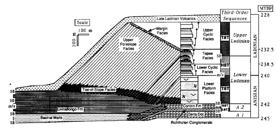
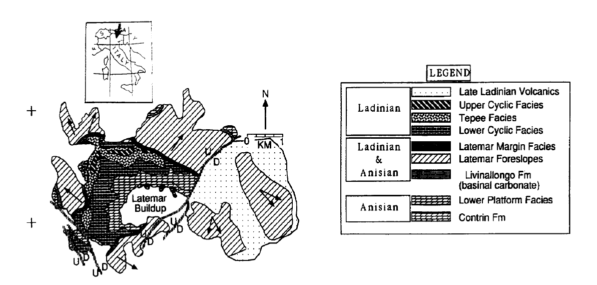
1. Geological setting
2. Cycles in the Latemar Limestone (space)
3. Potential origin of the Latemar cycles (time)
4. Testing the hypothesis: the data
5. Testing the hypothesis: the analysis

We acknowledge and respect the lək̓ʷəŋən peoples on whose traditional territory the university stands and the Songhees, Esquimalt and W̱SÁNEĆ peoples whose historical relationships with the land continue to this day.

import random
def pick_group(class_list):
    if len(class_list)>0:
        picked=random.sample(class_list,2)
        [class_list.remove(p) for p in picked]
        print(' and '.join(picked))
    else:
        picked=[]
    return class_list,picked

Geological setting

• why would a platformal setting be especially senstive to sea level changes?

class_list = ['Kai','Stacey','Grace','Liam','Matteo','Matthew','Noa','Izzy','Felix','Rhys','Andrea','Kristyn']
class_list,picked=pick_group(class_list)

Andrea and Kai

Geological setting

class_list = ['Kai','Stacey','Grace','Liam','Matteo','Matthew','Noa','Izzy','Felix','Rhys','Andrea','Kristyn']
class_list,picked=pick_group(class_list)

Grace and Rhys

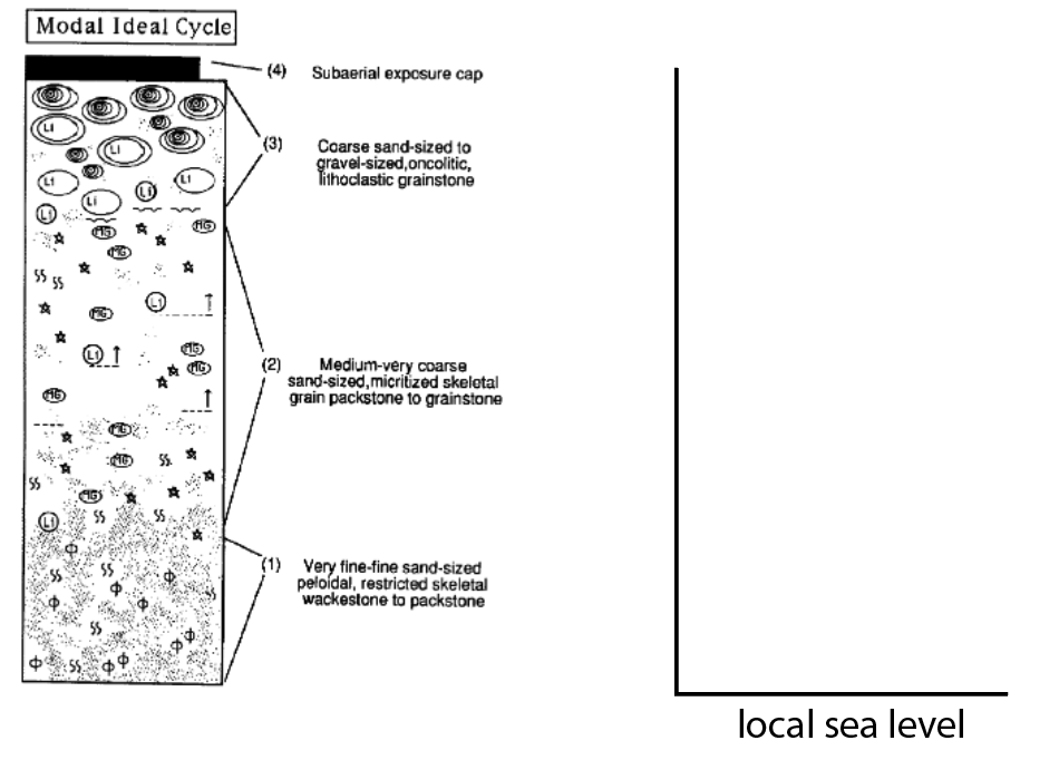
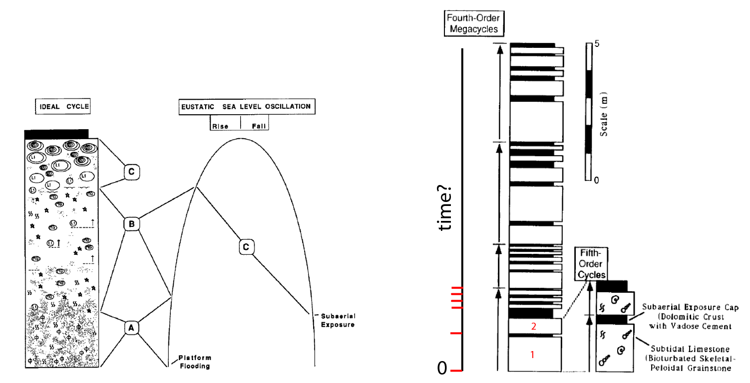
An ideal cycles in the Latemar Limestone

• what do the authors think is happening to sea level during deposition?
• "The absence of features indicating peritidal deposition between the subtidal member and vadose cap is conspicuous throughout the formation."

class_list = ['Stacey','Liam','Matteo','Matthew','Noa','Izzy','Felix','Kristyn']
class_list,picked=pick_group(class_list)

Izzy and Noa

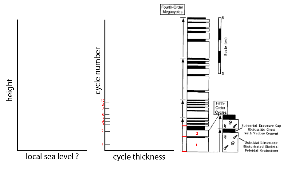
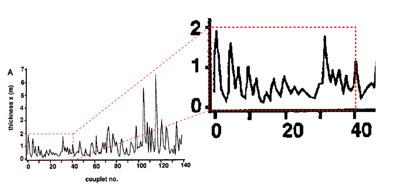
Nested cycles in the Latemar Limestone

• where is the ideal Latemar cycle on this plot?
• what is happening to cycle thickness up section?
• what do the authors think is happening to sea level?

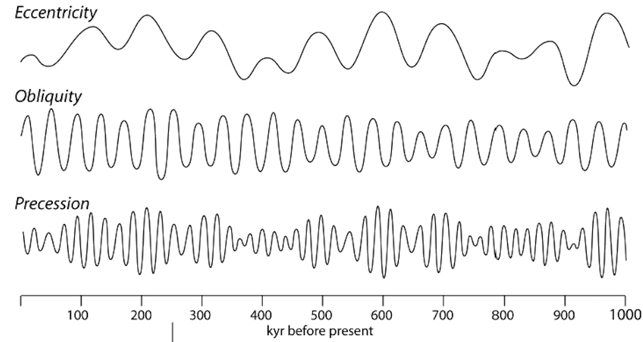
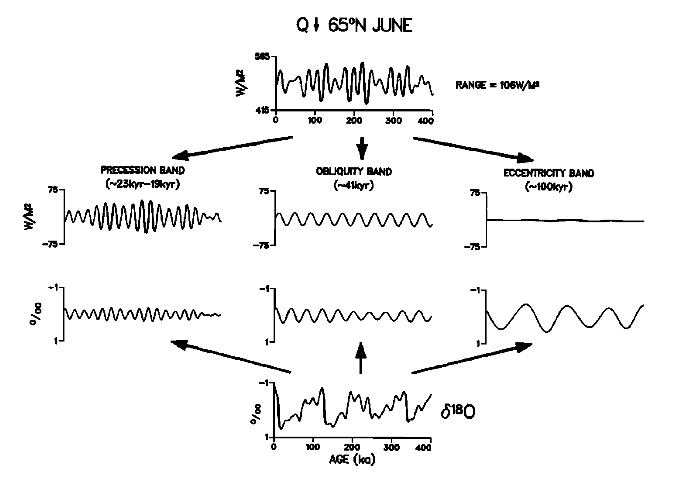
What is the propesed driver of cyclicity?

• what is driving an ideal cycle?
• what is driving the bundling of cycles into groups of five?

class_list = ['Stacey','Liam','Matteo','Matthew','Felix','Kristyn']
class_list,picked=pick_group(class_list)

Matthew and Matteo

But then why are the bundles asymmetric (according to the authors)?

class_list = ['Kai','Stacey','Grace','Liam','Matteo','Matthew','Noa','Izzy','Felix','Rhys','Andrea','Kristyn']
class_list,picked=pick_group(class_list)

class_list = ['Kai','Stacey','Grace','Liam','Matteo','Matthew','Noa','Izzy','Felix','Rhys','Andrea','Kristyn']
class_list,picked=pick_group(class_list)

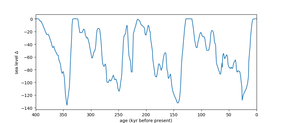
How then is time distributed in the Latemar succession?

• How long does one cycle last? How about 5 cycles?

Testing the hypothesis: how are they going to do it?

class_list = ['Stacey','Liam','Felix','Kristyn']
class_list,picked=pick_group(class_list)

Felix and Stacey

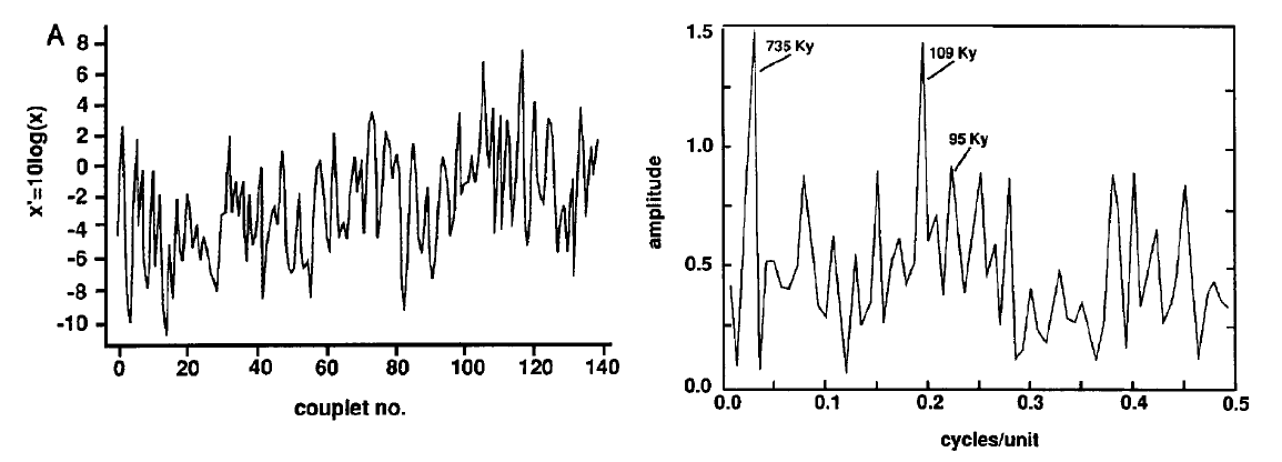
Testing the hypothesis: the analysis

Authors need to accomplish two things:

• show that a 5:1 bundling of cycles is a signicant feature of the data (easier)
  • in other words, are there cycles in space?
• make the case that 1 bundle = precession and 5 bundles = eccentricity (way, way harder)
  • do the cycles require a cyclic (in time) forcing?

Testing the hypothesis: the analysis

Overtones

#make some white noise
N=500
t = np.arange(0.0, 500, 1)
meas=scipy.signal.sawtooth((2*np.pi*t)/50)
mf=fft(meas - np.mean(meas))
tf,power,results=fft_axes(mf,N,N,1)
#plot
fig1=plt.figure(1,figsize=(27,6))
ax1=fig1.add_subplot(121)
ax1.set_xlabel('time')
ax1.set_ylabel('signal')
ax1.plot(meas,'-',lw=1,color='#6495ED')
ax1=fig1.add_subplot(122)
ax1.plot(tf,power,'-',lw=1,color='#6495ED')
ax1.set_xlabel('frequency (cycles per unit time)')
_=ax1.set_ylabel('power')

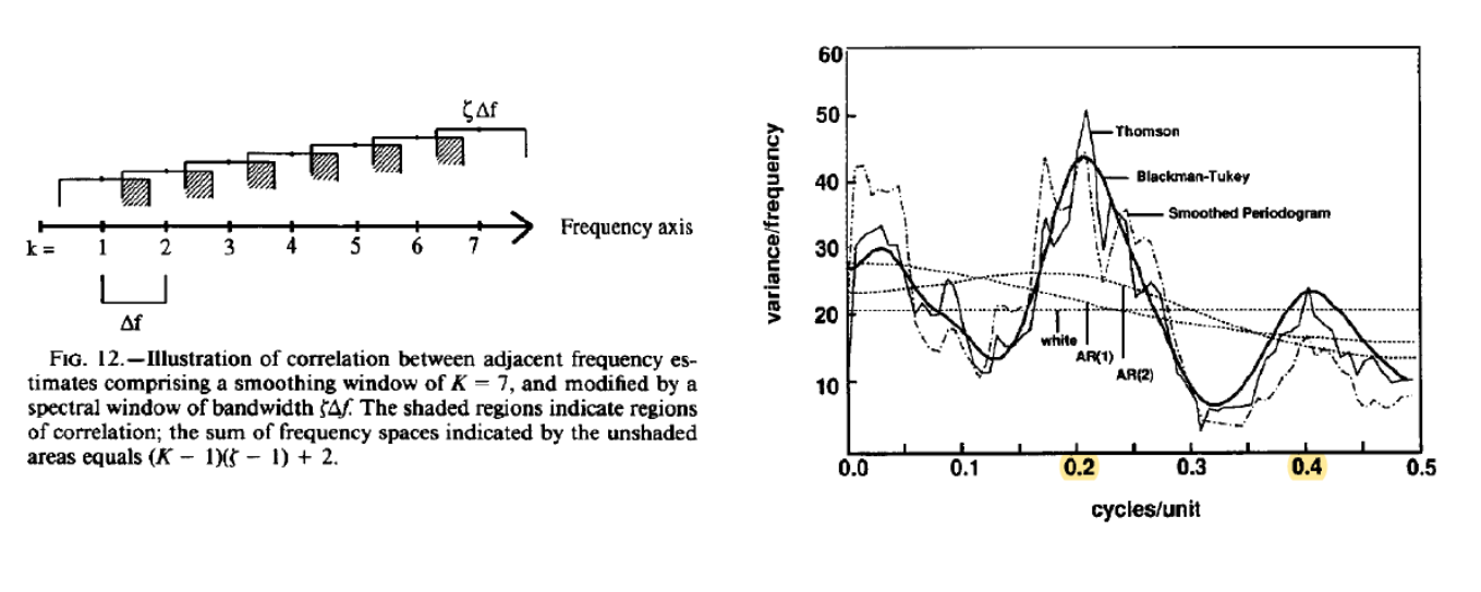
Noise: red or white?

Plotting help:

from scipy.fftpack import fft
import matplotlib.pyplot as plt
import numpy as np
from scipy import signal
import pandas as pd
import seaborn as sns
sns.set_context('talk')
%matplotlib inline

def fft_axes(yf,T,N,dt):
    
    if N % 2==0:
        xf=np.hstack((np.arange(0,1/(2*dt),1/T),(N//2)/T))
        power=2.0/N *np.abs(yf[0:len(xf)])
    else:
        xf=np.arange(0,1/(2*dt),1/T)
        power=2.0/N *np.abs(yf[0:len(xf)])
        
    results=pd.DataFrame(zip(xf,power),columns=['freq','power'])
    results=results.sort_values(by=['power'],ascending=False)

    return xf,power,results

Noise: red or white?

#make some white noise
N=500
t = np.arange(0.0, 500, 1)
meas=np.random.uniform(size=500)
#periodic signal
amp=0.0 #amp=0.065 #amp=0.13
ang_freq=0.02
meas=meas + amp*np.sin(ang_freq* 2*np.pi*t)
#fft
mf=fft(meas - np.mean(meas))
tf,power,results=fft_axes(mf,N,N,1)
#plot
fig1=plt.figure(1,figsize=(27,6))
ax1=fig1.add_subplot(121)
ax1.set_xlabel('time')
ax1.set_ylabel('signal')
ax1.plot(meas,'-',lw=1,color='#6495ED')
ax1=fig1.add_subplot(122)
ax1.plot(tf,power,'-',lw=1,color='#6495ED')
# ax1.annotate('our signal',(ang_freq,power[tf==ang_freq][0]),xytext=(50, 0), textcoords='offset points',fontsize=16,arrowprops=dict(arrowstyle="->"))
ax1.set_xlabel('frequency (cycles per unit time)')
_=ax1.set_ylabel('power')

Noise: red or white?

#make some red noise
t = np.arange(0.0, 500, 1)
meas=np.random.randint(-1,2,500)
meas=np.cumsum(meas)
#periodic signal
amp=2 #amp=2
ang_freq=0.02
meas=meas + amp*np.sin(ang_freq * 2*np.pi*t)
#fft
mf=fft(meas - np.mean(meas))
tf,power,results=fft_axes(mf,N,N,1)
#plot
fig1=plt.figure(1,figsize=(27,6))
ax1=fig1.add_subplot(121)
ax1.set_xlabel('time')
ax1.plot(meas,'-',lw=1,color='#6495ED')
ax1=fig1.add_subplot(122)
# ax1.plot(tf,power,'-',lw=1,color='#6495ED')
ax1.plot(np.log10(tf[1:]),np.log10(power[1:]),'-',lw=1,color='#6495ED')
# ax1.annotate('our signal',(np.log10(ang_freq),np.log10(power[tf==ang_freq][0])),xytext=(50, 0), textcoords='offset points',fontsize=16,arrowprops=dict(arrowstyle="->"))
ax1.set_xlabel('frequency (cycles per unit time)')
_=ax1.set_ylabel('power')     

#make some white noise
N=100
t = np.linspace(0.0, N, 100000)
meas=2*np.sin((2*np.pi*t)/50)+np.cos(2*np.pi*t/10)

#plot
fig1=plt.figure(1,figsize=(27,6))
plt.plot(t,meas+t/5)

[<matplotlib.lines.Line2D at 0x7f68c9294190>]