Lecture 14: Introduction to Age Models
- The importance of knowing time
- Building an age model
- Markov chain Monte Carlo approaches
- constant sedimentation rates
- varying sedimentation rates
We acknowledge and respect the lək̓ʷəŋən peoples on whose traditional territory the university stands and the Songhees, Esquimalt and W̱SÁNEĆ peoples whose historical relationships with the land continue to this day.
Importance of knowing time
Importance of knowing time
Age models are important: how do we get them?
- Cyclostratigraphy
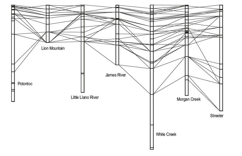
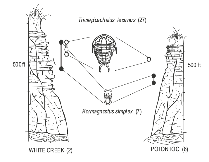
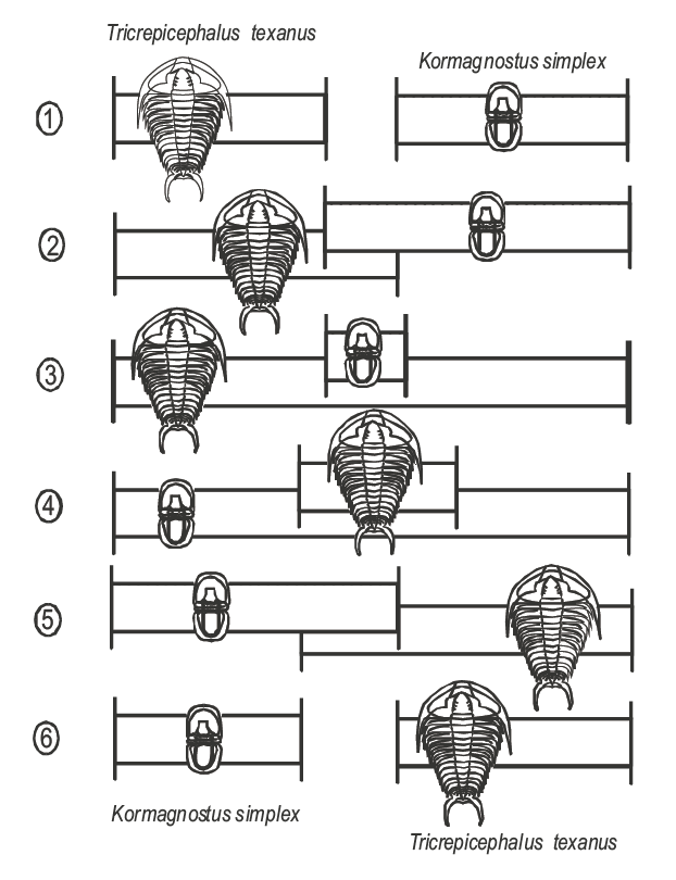
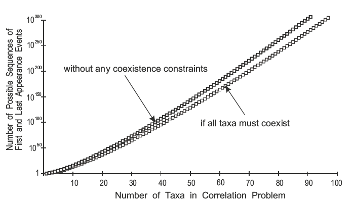
- Biostratigraphy
- Absolute ages
- U-Pb (volcanics), Ar-Ar (volcanics), Re-Os (sediments)
- Signal matching
- magnetostratigraphy
- chemostratigraphy
Building an age model
Building an age model
In [10]:
fig=plt.figure(1,figsize=(15,6))
ax=fig.add_subplot(121)
ax,trace,boxes,liths=rando_strat(ax,num_box=5,height=2,boxes=[],liths=[]) #stratigraphy for fun
#ashes in the strat column
for a in ashes:
    tmp_w=trace[(trace[:,0]<=ashes[a]['height']) & (trace[:,1]>ashes[a]['height']),2]
    ax.plot([0,tmp_w],[ashes[a]['height'],ashes[a]['height']],'r--')
#KT boundary
tmp_w=trace[(trace[:,0]<=KT) & (trace[:,1]>KT),2]
ax.plot([0,tmp_w],[KT,KT],'k--')
ax.text(tmp_w,KT,'  KT boundary',verticalalignment='center',fontsize=20)
#ash ages
ax=fig.add_subplot(122)
for a in ashes:
    ax.plot(ashes[a]['age'],ashes[a]['height'],'rs')
ax.plot([66.2,65.95],[KT,KT],'k--')
ax.set_xlim([66.2,65.95]); ax.set_ylim([-0.1,2])
ax.set_ylabel('meters'); _=ax.set_xlabel('age (Ma)')

Building an age model
In [11]:
fig=plt.figure(1,figsize=(15,6))
ax=fig.add_subplot(121)
ax,trace,boxes,liths=rando_strat(ax,num_box=5,height=2,boxes=boxes,liths=liths) #stratigraphy for fun
#ashes in the strat column
for a in ashes:
    tmp_w=trace[(trace[:,0]<=ashes[a]['height']) & (trace[:,1]>ashes[a]['height']),2]
    ax.plot([0,tmp_w],[ashes[a]['height'],ashes[a]['height']],'r--')
#KT boundary
tmp_w=trace[(trace[:,0]<=KT) & (trace[:,1]>KT),2]
ax.plot([0,tmp_w],[KT,KT],'k--')
#ash ages
ax=fig.add_subplot(122)
ash_table=np.array([(ashes[a]['age'],ashes[a]['height']) for a in ashes])
ax.plot(ash_table[:,0],ash_table[:,1],'rs-',lw=0.5)
#calculate KT age
KT_age=calc_age(ash_table,KT)
ax.plot([66.2,KT_age],[KT,KT],'k--')
ax.plot([KT_age,KT_age],[KT,KT],'w*',mec='k',markersize=20)
ax.text(KT_age,KT,'   %2.2f Ma.' % (KT_age),horizontalalignment='left',verticalalignment='center',fontsize=20)
ax.set_xlim([66.2,65.95]); ax.set_ylim([-0.1,2]); ax.set_ylabel('meters'); _=ax.set_xlabel('age (Ma)')

Building an age model
In [13]:
fig=plt.figure(1,figsize=(15,6))
ax=fig.add_subplot(121)
ax,trace,boxes,liths=rando_strat(ax,num_box=5,height=2,boxes=boxes,liths=liths) #stratigraphy for fun
#ashes in the strat column
for a in ashes:
    tmp_w=trace[(trace[:,0]<=ashes[a]['height']) & (trace[:,1]>ashes[a]['height']),2]
    ax.plot([0,tmp_w],[ashes[a]['height'],ashes[a]['height']],'r--')
#KT boundary
tmp_w=trace[(trace[:,0]<=KT) & (trace[:,1]>KT),2]
ax.plot([0,tmp_w],[KT,KT],'k--')
#ash ages
ax=fig.add_subplot(122)
for a in ashes:
    ax.plot(ashes[a]['age'],ashes[a]['height'],'rs')
    ax.plot([ashes[a]['age']+ashes[a]['2sd'],ashes[a]['age']-ashes[a]['2sd']],
            [ashes[a]['height'],ashes[a]['height']],'r-')
ax.plot([66.2,65.95],[KT,KT],'k--')
ax.set_xlim([66.2,65.95]); ax.set_ylim([-0.1,2]); ax.set_ylabel('meters');_=ax.set_xlabel('age (Ma)')

Building an age model
In [23]:
fig=plt.figure(1,figsize=(15,6))
ax=fig.add_subplot(121)
ax,trace,boxes,liths=rando_strat(ax,num_box=5,height=2,boxes=boxes,liths=liths) #stratigraphy for fun
#ashes in the strat column
for a in ashes:
    tmp_w=trace[(trace[:,0]<=ashes[a]['height']) & (trace[:,1]>ashes[a]['height']),2]
    ax.plot([0,tmp_w],[ashes[a]['height'],ashes[a]['height']],'r--')
#ash ages as distributions
ax=fig.add_subplot(122)
for a in ashes:
    #normal distribution
    mu=ashes[a]['age']
    sigma=ashes[a]['2sd']/2
    x = np.linspace(mu - 3*sigma, mu + 3*sigma, 300)
    #scaled for display
    distro=stats.norm.pdf(x, mu, sigma)
    distro=distro/max(distro)*0.3
    ax.plot(x, distro+ashes[a]['height'],'r')
    #ash strat height
    ax.plot([ashes[a]['age']+ashes[a]['2sd']*3/2,ashes[a]['age']-ashes[a]['2sd']*3/2],
            [ashes[a]['height'],ashes[a]['height']],'r--',lw=0.5)
ax.plot([66.2,65.95],[KT,KT],'k--')
ax.set_xlim([66.2,65.95]); ax.set_ylim([-0.1,2]); ax.set_ylabel('meters'); _=ax.set_xlabel('age (Ma)')

Building an age model
In [24]:
fig=plt.figure(1,figsize=(15,6))
ax=fig.add_subplot(121)
ax,trace,boxes,liths=rando_strat(ax,num_box=5,height=2,boxes=boxes,liths=liths) #stratigraphy for fun
for a in ashes:
    tmp_w=trace[(trace[:,0]<=ashes[a]['height']) & (trace[:,1]>ashes[a]['height']),2]
    ax.plot([0,tmp_w],[ashes[a]['height'],ashes[a]['height']],'r--')
#picking ages from distributions
ax=fig.add_subplot(122)
for a in ashes:
    mu=ashes[a]['age']
    sigma=ashes[a]['2sd']/2
    x = np.linspace(mu - 3*sigma, mu + 3*sigma, 300)
    distro=stats.norm.pdf(x, mu, sigma)
    pick=np.random.normal(mu,sigma,1)
    pick_distro=stats.norm.pdf(pick, mu, sigma)
    pick_distro=pick_distro/max(distro)*0.3
    distro=distro/max(distro)*0.3
    ax.plot(x, distro+ashes[a]['height'],'r')
    ax.plot([ashes[a]['age']+ashes[a]['2sd']*3/2,ashes[a]['age']-ashes[a]['2sd']*3/2],
            [ashes[a]['height'],ashes[a]['height']],'r--',lw=0.5)
    ax.plot(pick, pick_distro+ashes[a]['height'],'r*',mec='k',markersize=20)
ax.plot([66.2,65.95],[KT,KT],'k--')
ax.set_xlim([66.2,65.95]); ax.set_ylim([-0.1,2]); ax.set_ylabel('meters'); _=ax.set_xlabel('age (Ma)')

Building an age model
In [26]:
fig=plt.figure(1,figsize=(15,6))
ax=fig.add_subplot(121)
ax,trace,boxes,liths=rando_strat(ax,num_box=5,height=2,boxes=boxes,liths=liths) #stratigraphy for fun
#ashes in the strat column
for a in ashes:
    tmp_w=trace[(trace[:,0]<=ashes[a]['height']) & (trace[:,1]>ashes[a]['height']),2]
    ax.plot([0,tmp_w],[ashes[a]['height'],ashes[a]['height']],'r--')
ax=fig.add_subplot(122)
for a in ashes:
    ax.plot([ashes[a]['age']+ashes[a]['2sd'],ashes[a]['age']-ashes[a]['2sd']],
            [ashes[a]['height'],ashes[a]['height']],'r-')
#plot ten paths
np.random.shuffle(paths) #shuffle the deck
for p in paths[0:100]:
    ax.plot(p,[ashes[a]['height'] for a in ashes],'r-',lw=0.5)
#plot MCMC KT age
ax.plot([np.mean(KT_ages)+np.std(KT_ages)*2,np.mean(KT_ages)-np.std(KT_ages)*2],
        [KT,KT],'k-')

ax.plot([np.mean(KT_ages),np.mean(KT_ages)],[KT,KT],'w*',mec='k',markersize=20)
ax.text(np.mean(KT_ages)-np.std(KT_ages)*2,KT,r'   %2.2f$\pm$%2.2f Ma.' % (np.mean(KT_ages),np.std(KT_ages)*2),
        horizontalalignment='left',verticalalignment='center',fontsize=15)
ax.set_xlim([66.2,65.95]); ax.set_ylim([-0.1,2]); ax.set_ylabel('meters'); _=ax.set_xlabel('age (Ma)')

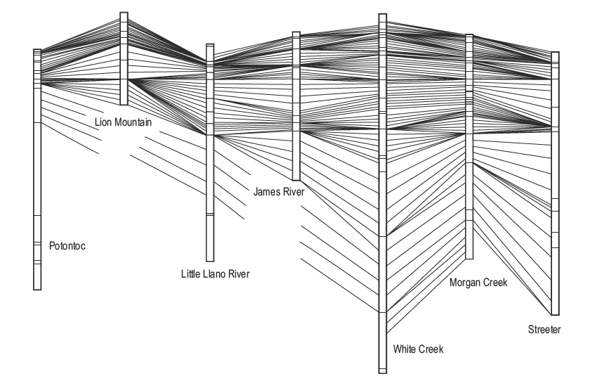
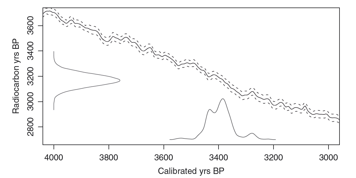
Power of Markov Chain Monte Carlo approaches
- prior distributions need not be Gaussian (figure from Haslett and Parnell, 2008)
How many samples is enough?
In [64]:
fig=plt.figure(1,figsize=(15,6))
ax=fig.add_subplot(111)
idx=list(range(1000)) +list(range(1000,len(KT_ages)+1,100))
#statistics of KT age as function of number of trials
KT_evolve=[]
for i in idx:
    KT_evolve.append((np.mean(KT_ages[0:i+1]),np.std(KT_ages[0:i+1]),len(KT_ages[0:i+1])))
KT_evolve=np.array(KT_evolve)
#plot the results
ax.plot(KT_evolve[:,2],KT_evolve[:,0],'r-',label='mean age')
ax.fill_between(KT_evolve[:,2],KT_evolve[:,0]+KT_evolve[:,1],KT_evolve[:,0]-KT_evolve[:,1],
                color='k',alpha=0.5,zorder=0,label='mean +/- 2s.d.')
ax.set_ylabel('age (Ma.)'); ax.set_xlabel('number of trials');_=ax.legend(loc='best')

Constant sedimentation rate assumption
In [29]:
def make_path(pts,g_shape,g_scale,delta):
    #separate a number of points (X) along a [0,1] path
    if pts!=0:
        #X numbers are drawn from a gamma distribution (G)
        #--> these represent the distances between successive points
        path=np.cumsum(np.random.gamma(g_shape,g_scale, pts))
    else:
        path=[1]#if X = 0, then path is simply [0,1]
    path=np.hstack((0,path))#add 0 as the path beginning
    #scale first to be between 0 and 1, and then 0 to delta
    path=path/path[-1]*delta
    return(path)

fig=plt.figure(1,figsize=(6,6)); ax=fig.add_subplot(111)
#assumes constant sedimentation rate between anchors
ax.plot([0,1],[0,1],'-s');ax.set_xlabel('change in time'); _=ax.set_ylabel('change in height')

Constant sedimentation rate assumption
In [103]:
fig=plt.figure(1,figsize=(6,6)); ax=fig.add_subplot(111);
ax.set_xlabel('change in time'); _=ax.set_ylabel('change in height')
num_paths=200 #add knots to the path
for i in range(num_paths):
    pts=np.random.poisson(5, 1)[0] #discrete integer
    t_path=make_path(pts,1,1,1) #age change between knots
    h_path=make_path(pts,1,1,1) #position change between knots
    ax.plot([0]+list(np.cumsum([1/pts]*pts)),[0]+list(np.cumsum([1/pts]*pts)),'-s')
#     ax.plot(t_path,h_path,'-s') #plot the path
    #plot many paths
    ax.plot(t_path,h_path,'k-',lw=0.5,alpha=0.25)

Constant sedimentation rate assumption
In [ ]:
...
for i in range(num_paths):
    pts=np.random.poisson(5, 1)[0] #discrete integer
    ...
Poisson distribution is a discrete probability distribution that expresses the probability of a given number of events occurring in a fixed interval of time or space if these events occur with a known constant mean rate and independently of the time since the last event.
Exponential distribution is the probability distribution of the time between events in a Poisson point process
In [22]:
import numpy as np
from matplotlib import pyplot as plt
import seaborn as sns
fig=plt.figure(figsize=(10,10))
a = np.random.uniform(0,1,100000)
b = a<0.1
sns.kdeplot(np.diff(np.where(b)[0]),color=sns.color_palette('deep')[2],fill=True,lw=3)
c = np.random.exponential(10,100000)
sns.kdeplot(c,color=sns.color_palette('deep')[1],fill=True,lw=3)
sns.despine()

Deciding on number of sedimentation rate changes
In [67]:
#number of timesteps
t=200000
#probability of change
prob=0.25
#start with sediment on
state=1
#switch state
sed=np.array([state*-1 if np.random.random()<prob else state for i in range(t)])
#plot the sedimentation rate history
fig=plt.figure(1,figsize=(25,7.5));ax=fig.add_subplot(111)
#plot as timeseries
ax.plot(sed[0:100]); ax.set_ylabel('sediment switch'); _=ax.set_xlabel('time')

Deciding on number of sedimentation rate changes
In [60]:
sns.histplot(np.random.poisson(1,10000),
             binwidth=1)
_=plt.gca().set_xlabel("discrete events over an interval of time")

In [71]:
sns.histplot(np.random.exponential(1,10000))
_=plt.gca().set_xlabel('interval of time between events')
# plt.gca().set_yscale('log')

Deciding on number of sedimentation rate changes
In [73]:
fig=plt.figure(1,figsize=(7.5,7.5)); ax=fig.add_subplot(111);
ax.set_xlabel('change in time'); _=ax.set_ylabel('change in height')
num_paths=1 #add knots to the path
for i in range(num_paths):
    pts=np.random.poisson(5, 1)[0]
    #age change between knots
    t_path=make_path(pts,1,1,1)
    #position change between knots
    h_path=make_path(pts,1,1,1)
#     #plot the knot number
#     ax.plot([0]+list(np.cumsum([1/pts]*pts)),[0]+list(np.cumsum([1/pts]*pts)),'-s')
    #plot the path
    ax.plot(t_path,h_path,'-s')

Picking sedimentation rates
In [71]:
fig=plt.figure(1, figsize=(12,6)); ax=fig.add_subplot(111)
g_shape=1.5; g_loc=0; g_scale=1
gam_hist=np.random.gamma(g_shape,g_scale, 10000) #10K draws with shape = 1.5 and scale = 1
x=np.linspace(0,max(gam_hist),1000)
gam=stats.gamma.pdf(x,g_shape,g_loc,g_scale) #continuous function
ax.hist(gam_hist,density=True,alpha=0.75,color='#6495ED',
        label=r'$\lambda$ = %2.1f; $\mu$ = %2.3f' % (g_shape*g_scale,np.mean(gam_hist))); ax.plot(x,gam,'k--')
g_shape=10.5; g_loc=0; g_scale=1 #10K draws with shape = 10.5 and scale = 1
gam_hist=np.random.gamma(g_shape,g_scale, 10000)
x=np.linspace(0,max(gam_hist),1000); gam=stats.gamma.pdf(x,g_shape,g_loc,g_scale) #continuous function
ax.hist(gam_hist,density=True,alpha=0.75,color='#B22222',
        label=r'$\lambda$ = %2.1f; $\mu$ = %2.3f' % (g_shape*g_scale,np.mean(gam_hist))); ax.plot(x,gam,'k--')
#plot labels
ax.set_title('examples of gamma distributions')
ax.legend(); _=ax.text(0.99,0.725,', '.join(['%2.3f' %(g) for g in gam_hist[0:6].tolist()]) + ', ... ',
                       transform=ax.transAxes,horizontalalignment='right',fontsize=15)

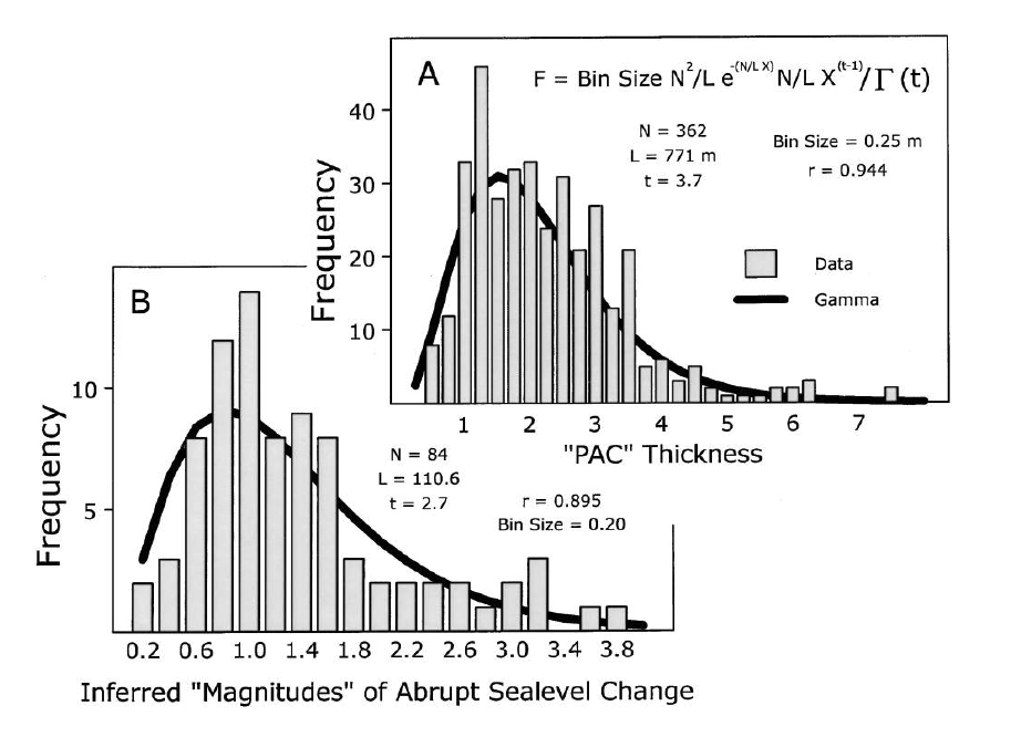
gamma distributions in sedimentology
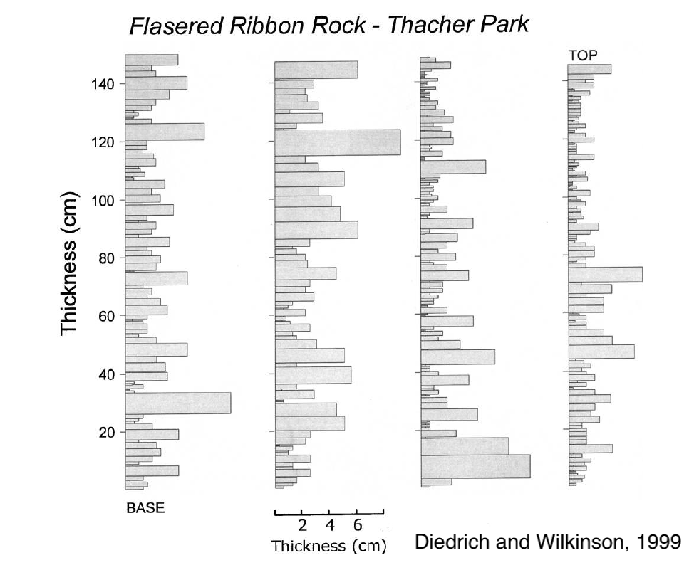
gamma distributions in sedimentology
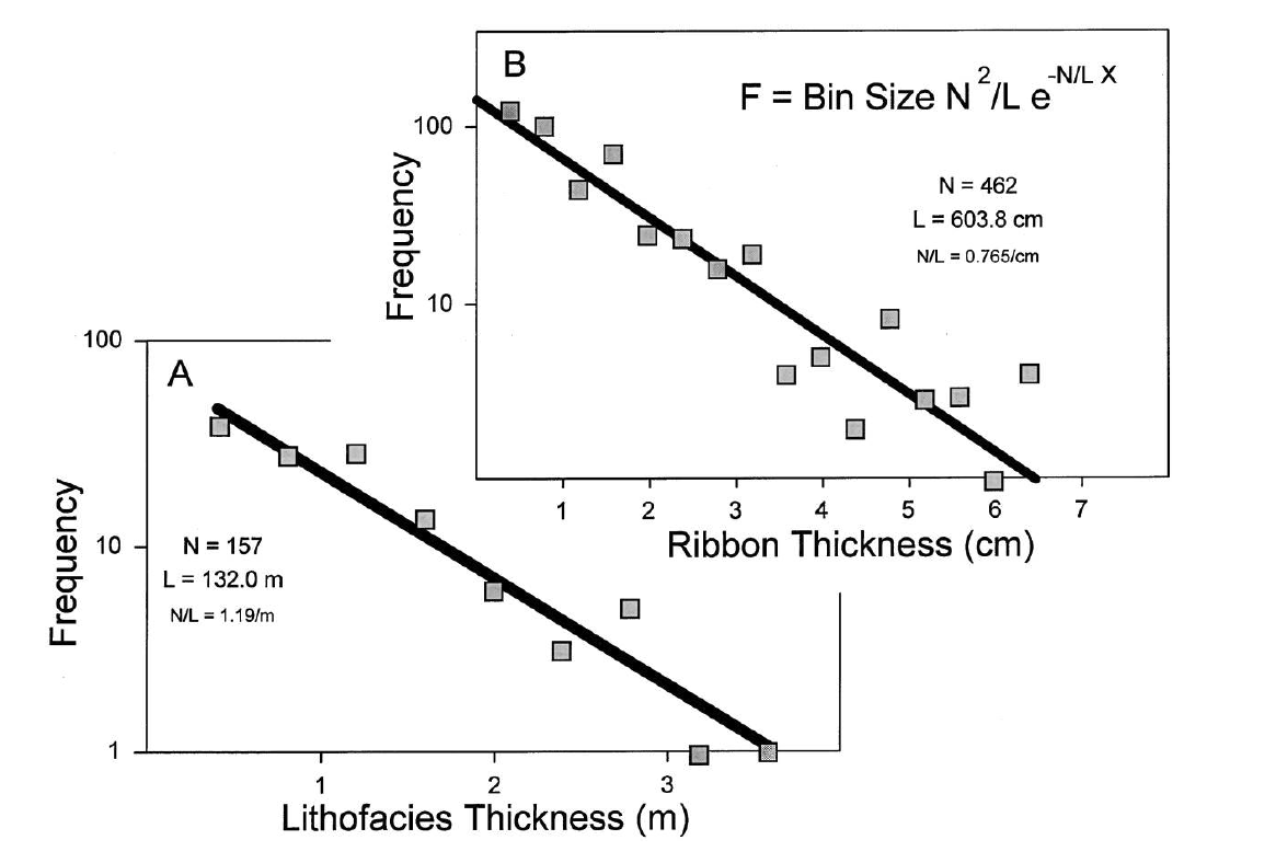
gamma distributions in sedimentology
compound Poisson gamma age models
In [90]:
fig=plt.figure(1,figsize=(7.5,7.5)); ax=fig.add_subplot(111);
ax.set_xlabel('change in time'); _=ax.set_ylabel('change in height')
num_paths=200 #add knots to the path
for i in range(num_paths):
    pts=np.random.poisson(5, 1)[0]
    #age change between knots
    t_path=make_path(pts,1,1,1)
    #position change between knots
    h_path=make_path(pts,1,1,1)
#     #plot the knot number
#     ax.plot([0]+list(np.cumsum([1/pts]*pts)),[0]+list(np.cumsum([1/pts]*pts)),'-s')
    #plot the path
    ax.plot(t_path,h_path,'k-',lw=0.5,alpha=0.25)
_=ax.plot(t_path,h_path,'-s')

compound Poisson gamma age models
In [91]:
import pandas as pd
import time
#local way to load data
sluggan=[{'position': 44.5, 'age': 985.0, '2sd': 45.0}, {'position': 49.5, 'age': 1225.0, '2sd': 65.0},
        {'position': 69.0, 'age': 1635.0, '2sd': 75.0}, {'position': 102.0, 'age': 2130.0, '2sd': 45.0},
        {'position': 125.0, 'age': 2930.0, '2sd': 85.0}, {'position': 165.0, 'age': 3945.0, '2sd': 85.0},
        {'position': 185.0, 'age': 4180.0, '2sd': 90.0}, {'position': 232.5, 'age': 4556.666667, '2sd': 76.66666667},
        {'position': 239.0, 'age': 4965.0, '2sd': 75.0}, {'position': 272.5, 'age': 5320.0, '2sd': 65.0},
        {'position': 297.5, 'age': 6760.0, '2sd': 90.0}, {'position': 332.0, 'age': 7855.0, '2sd': 115.0},
        {'position': 367.5, 'age': 8176.666667, '2sd': 65.0},{'position': 407.0, 'age': 8540.0, '2sd': 120.0},
        {'position': 427.0, 'age': 9360.0, '2sd': 150.0},{'position': 447.5, 'age': 9475.0, '2sd': 145.0},
        {'position': 461.0, 'age': 9610.0, '2sd': 130.0},{'position': 484.5, 'age': 10805.0, '2sd': 125.0},
        {'position': 499.0, 'age': 10995.0, '2sd': 160.0},{'position': 509.0, 'age': 11625.0, '2sd': 160.0},
        {'position': 518.0, 'age': 12265.0, '2sd': 125.0}]
print('number of ages: %s' %(len(sluggan)))
#convert list of dictionaries into a DataFrame
sluggan=pd.DataFrame(sluggan)
sluggan['position']=sluggan['position']*-1
sluggan=sluggan.sort_values(by='position')
sluggan=sluggan.reset_index()
sluggan.head()
number of ages: 21
Out[91]:
| index | position | age | 2sd | |
|---|---|---|---|---|
| 0 | 20 | -518.0 | 12265.0 | 125.0 |
| 1 | 19 | -509.0 | 11625.0 | 160.0 |
| 2 | 18 | -499.0 | 10995.0 | 160.0 |
| 3 | 17 | -484.5 | 10805.0 | 125.0 |
| 4 | 16 | -461.0 | 9610.0 | 130.0 |
compound Poisson gamma age models
compound Poisson gamma age models
In [96]:
fig=plt.figure(1,figsize=(12,6)); ax=fig.add_subplot(111)
#randomly pick ~100 age models (could be less)
idx=np.random.randint(len(true_paths))
for a in true_paths[idx:idx+100]:
    ax.plot(a[:,0],a[:,1]/100,'-',lw=0.5)
#statistics on interpolated ages
# ax.fill_betweenx(path_stats['position']/100,path_stats['2.5'],path_stats['97.5'],
#                 color='k',edgecolor='none',alpha=0.3,zorder=0)
#plot the median age (constant sed rate)
# ax.plot(path_stats['50'],path_stats['position']/100,'k--',lw=1)
#plot age constraints
# for i,a in sluggan.iterrows():
#     ax.plot([a['age']+a['2sd'],a['age']-a['2sd']],[a['position']/100,a['position']/100],'k-',lw=2)
#plot age of demo horizon
# ax.plot([demo['age']+demo['2sd'],demo['age']-demo['2sd']],[demo['position']/100,demo['position']/100],'r-',lw=2)
#plot labels
ax.set_xlim([13000,0]); ax.set_xlabel('age (years BP)');_=ax.set_ylabel('depth (m)')

compound Poisson gamma age models
In [99]:
#RUN AGE MODEL FOR KT U-Pb DATA
tic=time.time()
#pick self-consistent ages (based on Markov Chain Monte Carlo)
num_trials=1000
KT_picks=age_pick(KTashes,num_trials)
#define lambda for poisson draws
#NB: if lambda=0, "constant sed rate model" is result
p_lam=0
p_lam=10.5
#define shape and scale for gamma draws
#NB: age model only sensitive to shape
g_shape=1.5
g_scale=1\
#number of interpolation points per age anchor
num_interp=1000
#run compound Poission-Gamma age model
true_paths,interp_paths,path_stats,age_models = make_age_model(KTashes,KT_picks,p_lam,g_shape,g_scale,num_interp)
#age of KT Boundary
KT={'position':0.6,
       'age': np.mean([a(0.6) for a in age_models]),
        '2sd': 2*np.std([a(0.6) for a in age_models])}
toc=time.time()
print(r'number of trials: %s' %(num_trials))
print(r'model run time: %2.2f seconds' % (toc-tic))
print(r'age of KT boundary produce by model: %2.2f +/- %2.2f Ma.' %(KT['age'],KT['2sd']))
number of trials: 1000
model run time: 0.47 seconds
age of KT boundary produce by model: 66.08 +/- 0.04 Ma.
compound Poisson gamma age models
In [100]:
fig=plt.figure(1,figsize=(12,6)); gs = fig.add_gridspec(1,4); ax=fig.add_subplot(gs[0])
ax,trace,boxes,liths=rando_strat(ax,num_box=5,height=2,boxes=boxes,liths=liths) #stratigraphy for fun
ax=fig.add_subplot(gs[1:])
#statistics on interpolated ages
ax.fill_betweenx(path_stats['position'],path_stats['2.5'],path_stats['97.5'],color='k',edgecolor='none',alpha=0.3,zorder=0)
#plot age constraints
for i,a in KTashes.iterrows():
    ax.plot([a['age']+a['2sd'],a['age']-a['2sd']],
            [a['position'],a['position']],'k-',lw=2)
#     ax.plot(np.mean(KT_picks[:,i]),a['position'],'r+',alpha=0.5,markersize=10)
#     ax.plot([np.mean(KT_picks[:,i])+2*np.std(KT_picks[:,i]),np.mean(KT_picks[:,i])-2*np.std(KT_picks[:,i])],
#            [a['position'],a['position']],'r-',lw=3,alpha=0.5)
#plot and label KT age
ax.text(KT['age']-KT['2sd'],KT['position'],'   %2.2f$\pm$%2.2f Ma.' % (KT['age'],KT['2sd']),fontsize=15,horizontalalignment='left',verticalalignment='center')
ax.plot([KT['age']+KT['2sd'],KT['age']-KT['2sd']],
        [KT['position'],KT['position']],'k--',lw=2); ax.plot(KT['age'],KT['position'],'w*',mec='k',markersize=20)
ax.set_xlim([66.2,65.95]);ax.set_xlabel('age (Ma.)');_=ax.set_ylabel('height (m)')

compound Poisson gamma age models
Appendix: more on gamma distributions in sedimentology
In [80]:
#timesteps; probability of change; starting state
t=20000; prob=0.25; state=1
#minimum beds in a parasequence
min_couplet_num=3

#switch state
sed=np.array([state*-1 if np.random.random()<prob else state for i in range(t)])
#find the "on" periods
on=np.where(sed==1)[0]

#find indices of consecutive "on" periods
on_breaks=list(np.where(np.diff(on)!=1)[0]+1)

#group into pairs
on_breaks=[0]+on_breaks+[len(on)]
on_breaks=list(zip(on_breaks[0:-1],on_breaks[1:]))

#calculate lengths of "sediment on" period
on_time=[]
for o in on_breaks:
    on_time.append(len(on[o[0]:o[1]]))

#here, the "on" periods are used to bundle couplets
#--> value = number of couplets
on_time=np.cumsum(np.array(on_time)+min_couplet_num-1)
couplet_idx=list(zip(list(on_time[0:-1]),list(on_time[1:])))
couplet_idx=[tuple((0, couplet_idx[0][0]))]+couplet_idx
#generate thickess of those couplets
couplets=np.random.gamma(1,1, couplet_idx[-1][1])
#package them up
bundles=[np.sum(couplets[i[0]:i[1]]) for i in couplet_idx]
Appendix: more on gamma distributions in sedimentology
In [81]:
#first hundred couplets for plotting
demo_couplets=list(np.cumsum(couplets)[0:100])
demo_couplets=[0]+demo_couplets
demo_couplets=list(zip(demo_couplets[0:-1],demo_couplets[1:]))
#make thickness vs. height boxes
couplet_boxes=[]
for d in demo_couplets:
    xy=np.array([(0,d[0]),(d[1]-d[0],d[0]),(d[1]-d[0],d[1]),(0,d[1])])
    rect = Polygon(xy,closed=True,facecolor="#"+''.join([np.random.choice([a for a in '0123456789ABCDEF']) for j in range(6)]))
    couplet_boxes.append(rect)
#bundles of couplets
demo_bundles=np.cumsum(bundles)[0:100]
demo_bundles=demo_bundles[demo_bundles<demo_couplets[-1][1]]
Appendix: more on gamma distributions in sedimentology
In [82]:
fig=plt.figure(1,figsize=(20,11)); ax=fig.add_subplot(121); ax.plot(sed[0:100],range(100)) #plot sedimentation history
ax.set_ylabel('time'); ax.set_xlabel('sediment switch'); ax.set_xticks([-1.0,1.0]); ax.set_xticklabels(['off','on'])
ax=fig.add_subplot(122); _=[ax.add_patch(r) for r in couplet_boxes] #plot bed thickness vs. height
ax.set_xlim([0,np.ceil(max(couplets[0:100]))]); ax.set_ylim([0,np.ceil(demo_couplets[-1][1])])
ax.set_ylabel('height (meters)');ax.set_xlabel('bed thickness (meters)')
_=[ax.plot(ax.get_xlim(),[d,d],'k--') for d in demo_bundles] #plot the parasequence boundaries
_=ax.text(ax.get_xlim()[1],demo_bundles[0],'parasequence top',horizontalalignment='right',verticalalignment='bottom',fontsize=15)

Appendix: more on gamma distributions in sedimentology
In [83]:
#histogram of bed thickness
fig=plt.figure(1,figsize=(20,11)); ax=fig.add_subplot(221)
ax.hist(couplets,bins=30,density=True); ax.set_xlabel('bed thickness (meters)')
#histogram of number of beds in a parasequence
ax=fig.add_subplot(222); ax.hist([i[1]-i[0] for i in couplet_idx],bins=30,density=True); ax.set_xlabel('beds per parasequence')
#histogram of parasequence thickness
ax=fig.add_subplot(212); ax.hist(bundles,bins=30,density=True);_=ax.set_xlabel('parasequence thickness (meters)')
