Lectures 15-16: Carbonates

1. Carbon cycle
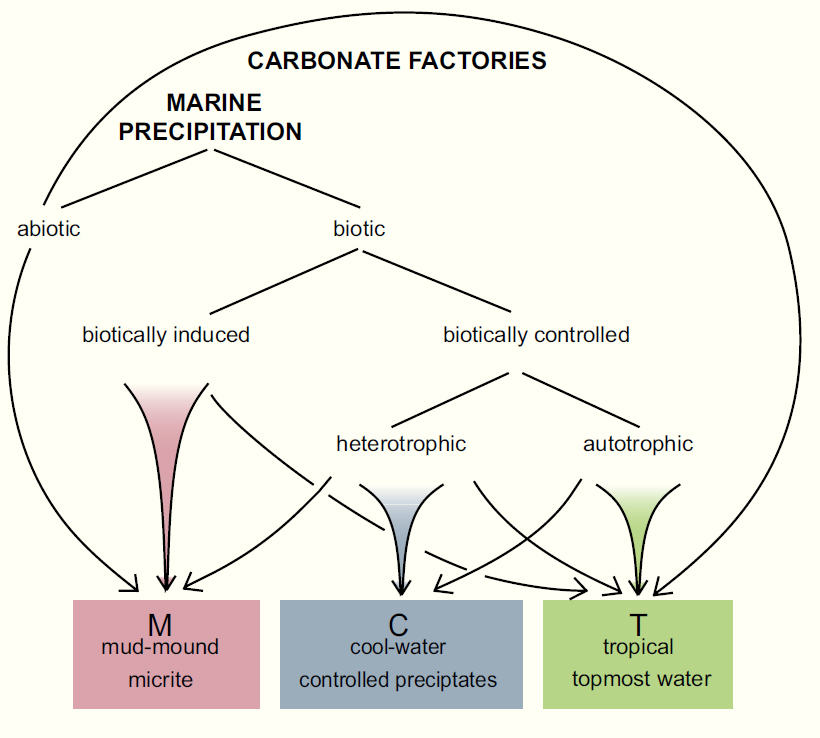
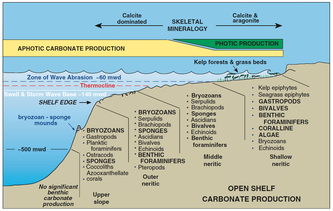
   1. Carbonate Factories
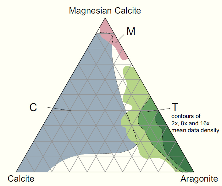
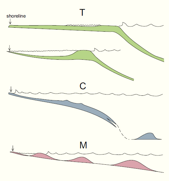
      1. T vs C vs M
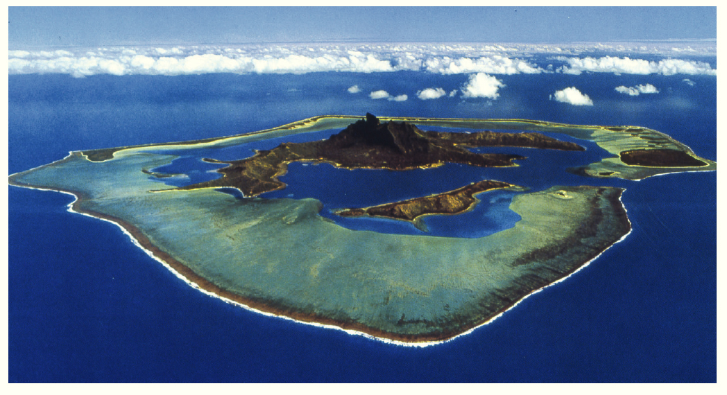
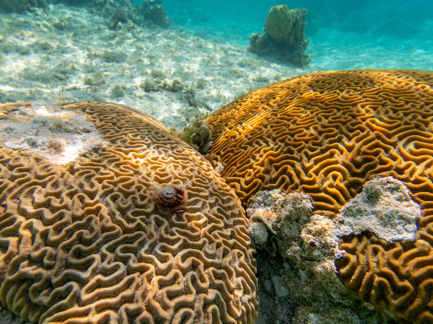
      2. Examples of each
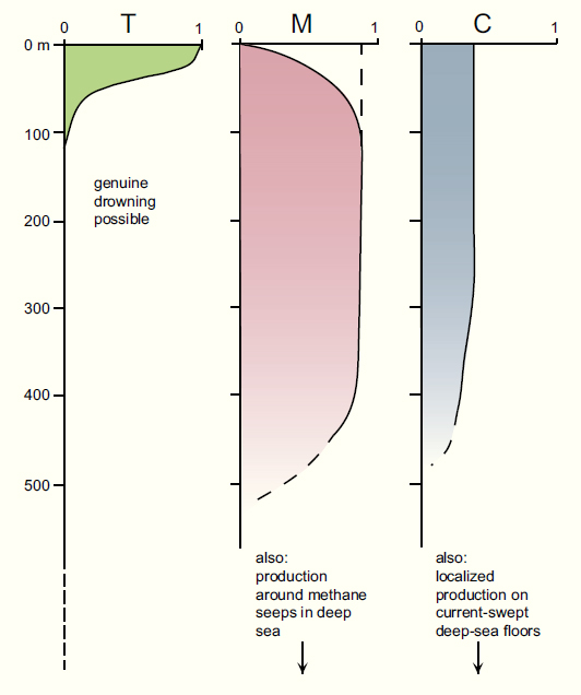
      3. Sedimentation rates and growth potential of each
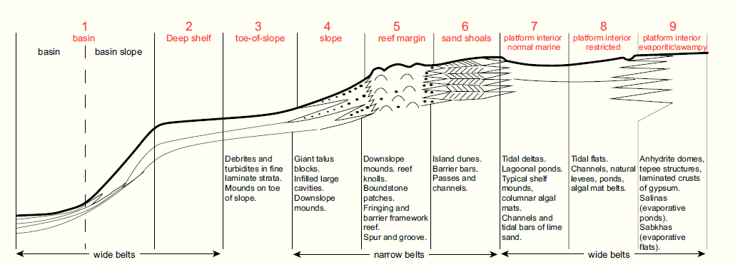
   2. Geometry of Carbonate Accumulations
   3. Modeling Carbonate Stratigraphy

We acknowledge and respect the lək̓ʷəŋən peoples on whose traditional territory the university stands and the Songhees, Esquimalt and W̱SÁNEĆ peoples whose historical relationships with the land continue to this day.

Introduction to final assignment concept.

(drawing on board)

Carbonates, the big picture:

(drawing on board)

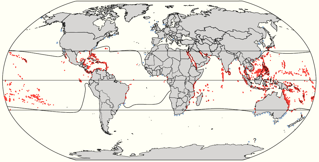
World Reef Map https://maps.lof.org/lof

import numpy as np
from matplotlib import pyplot as plt
%matplotlib inline
dz = np.linspace(0,100,1000)
extinction_coeff = 0.2
light_z = np.exp(-extinction_coeff*dz)
plt.plot(light_z,-dz,label='light')
light_base=.1
production_capacity = 1 
production_z = production_capacity * np.tanh(light_z/light_base)
plt.plot(production_z,-dz,label='carbonate production')
plt.gca().set_ylim([-40,0]); plt.legend(loc='best'); plt.gca().set_ylabel('depth (m)')

Text(0, 0.5, 'depth (m)')

plt.plot([0,1000],[0,0],label='sea level')
dx = np.linspace(0,1000,1000)
topography = np.zeros(1000)-200
topography[dx>300]=-10
topography[dx>700]=-200
plt.plot(dx,topography,label='topography')
plt.gca().set_ylabel('depth (m)');plt.legend(loc='best',fontsize=10)

<matplotlib.legend.Legend at 0x7f28c2d73510>

plt.plot(dx,prod_func(-topography),label='production\ncapacity')
plt.legend(loc='best',fontsize=10)

<matplotlib.legend.Legend at 0x7f28c19abc10>

from scipy.signal import gaussian
window_size = 50
standard_deviation = 10
plt.plot(gaussian(1+2*window_size,standard_deviation))

[<matplotlib.lines.Line2D at 0x7f28c2db5510>]

restriction = np.convolve(topography,gaussian(1+2*window_size,standard_deviation),mode='valid')
restriction -= np.min(restriction)
restriction /= 7000 #multiply to scale shelf production
productivity = prod_func(-topography)
plt.plot(dx,productivity,label='production\ncapacity')
productivity[window_size:-window_size]=productivity[window_size:-window_size]*(1-restriction)
plt.plot(dx,productivity,label='production\ncapacity\nrestriction')
plt.legend(loc='best',fontsize=10); plt.gca().set_ylabel('carbonate\nproduction')

Text(0, 0.5, 'carbonate\nproduction')

r = 1
capacity=2
N=.5
growth_rate = r*N*(1-N/capacity)

dt = 1  # timestep
base_level_rise = 100  # long term subsidence in meters
dx = 10  # x grid spacing
total_time = 3e6  # duration of simulation in years
initial_baselevel = 1  # in meters
sed_Q = 0.0  # sedimentation flux

#create an instance of Diffuse1D (defined above)
model = Diffuse1D(
    length=10000,
    spacing=dx,
    tstep=dt,
    left=0,
    right=0,
    K=2e-2,
    sed_Q=sed_Q,
    no_flux_boundary=True,
)

xt = np.linspace(0, total_time, 10000)  # creating uniform timegrid
RSL1 = -1.5 * np.sin(xt * 2 * np.pi * (1 / 20000))  # cyclic sea level component 1
RSL2 = 1 * sawtooth_wave(5, xt * 2 * np.pi * (1 / 100000))  # cyclic sea level component 2
RSL = (base_level_rise / (total_time) * xt + initial_baselevel)  # cyclic sea level + subsidence
# creates a function in the Diffuse1D model mapping your sea level boundary condition to time
model.set_baselevel(xt, RSL)

#to plot your model sea level boundary condition
plt.plot(xt/1000,model.base_level_fun(xt))
plt.gca().set_xlabel('Time (kilo-years)')
plt.gca().set_ylabel('Base level')

Text(0, 0.5, 'Base level')

plt.plot(model.u)
model.u=topography
plt.plot(model.u)
for i in tqdm(range(1000)):
    model.run_step()
plt.plot(model.u)

for i in tqdm(range(2000)):
    model.run_step()
plt.plot(model.u)
plt.gca().set_ylim([-50,0])

HBox(children=(FloatProgress(value=0.0, max=1000.0), HTML(value='')))

HBox(children=(FloatProgress(value=0.0, max=2000.0), HTML(value='')))

(-50, 0)

dt = 10  # timestep
base_level_rise = 60  # long term subsidence in meters
dx = 10  # x grid spacing
total_time = 1e6  # duration of simulation in years
initial_baselevel = 1  # in meters
sed_Q = 0.0  # sedimentation flux

#create an instance of Diffuse1D (defined above)
model = Diffuse1D(
    length=10000,
    spacing=dx,
    tstep=dt,
    left=0,
    right=0,
    K=2e-2,
    sed_Q=sed_Q,
    no_flux_boundary=True,
)

xt = np.linspace(0, total_time, 10000)  # creating uniform timegrid
RSL1 = 2 * np.sin(xt * 2 * np.pi * (1 / 1e5))  # cyclic sea level component 1
RSL = (base_level_rise / (total_time) * xt + initial_baselevel +RSL1)  # cyclic sea level + subsidence
# creates a function in the Diffuse1D model mapping your sea level boundary condition to time
model.set_baselevel(xt, RSL)
model.u=topography
model.carb_rate = .0015

#to plot your model sea level boundary condition
plt.plot(xt/1000,model.base_level_fun(xt))
plt.gca().set_xlabel('Time (kilo-years)')
plt.gca().set_ylabel('Base level')

Text(0, 0.5, 'Base level')

# initial lists to store model outputs throughout the simulation
beds = [] #model topography
age = [] #model time
rsl = [] #relative (local) sea level
sed_on = True
progress_bar = tqdm(range(int(total_time / dt / 1))) #run the model for the full duration, the tqdm wrapper provides a progress bar
for i in progress_bar:
    model.run_step() #run 1 timestep dt
    if i%50==0: #save every 50 steps to our lists
        beds.append(model.u)
        age.append(model.time)
        rsl.append(model.base_level)

HBox(children=(FloatProgress(value=0.0, max=100000.0), HTML(value='')))

skip=25
animate_beds(beds=beds[::skip],otime=age[::skip],rsl=rsl[::skip],aspect=2, ymin=-50, ymax=75, color=False)

column_number = 325
bed_facies, bed_bottom, bed_thickness, bed_colors = get_strat_column(beds, age, rsl, column_number, skip=10)
plot_column(bed_facies, bed_bottom, bed_thickness, bed_colors, left=column_number)
plt.gca().set_aspect(.05)

column_number = 500
bed_facies, bed_bottom, bed_thickness, bed_colors = get_strat_column(beds, age, rsl, column_number, skip=10)
plot_column(bed_facies, bed_bottom, bed_thickness, bed_colors, left=column_number)
plt.gca().set_aspect(.05)