Lecture 4: Sea-floor depth, age, and heat flow
- How do we map the seafloor today?
- Gravity, strain, and the geoid
- Stochastic reheating model
Mapping the sea-floor
Mapping the sea-floor
- A combination of:
- Depth Soundings
- Satellite Altimetry
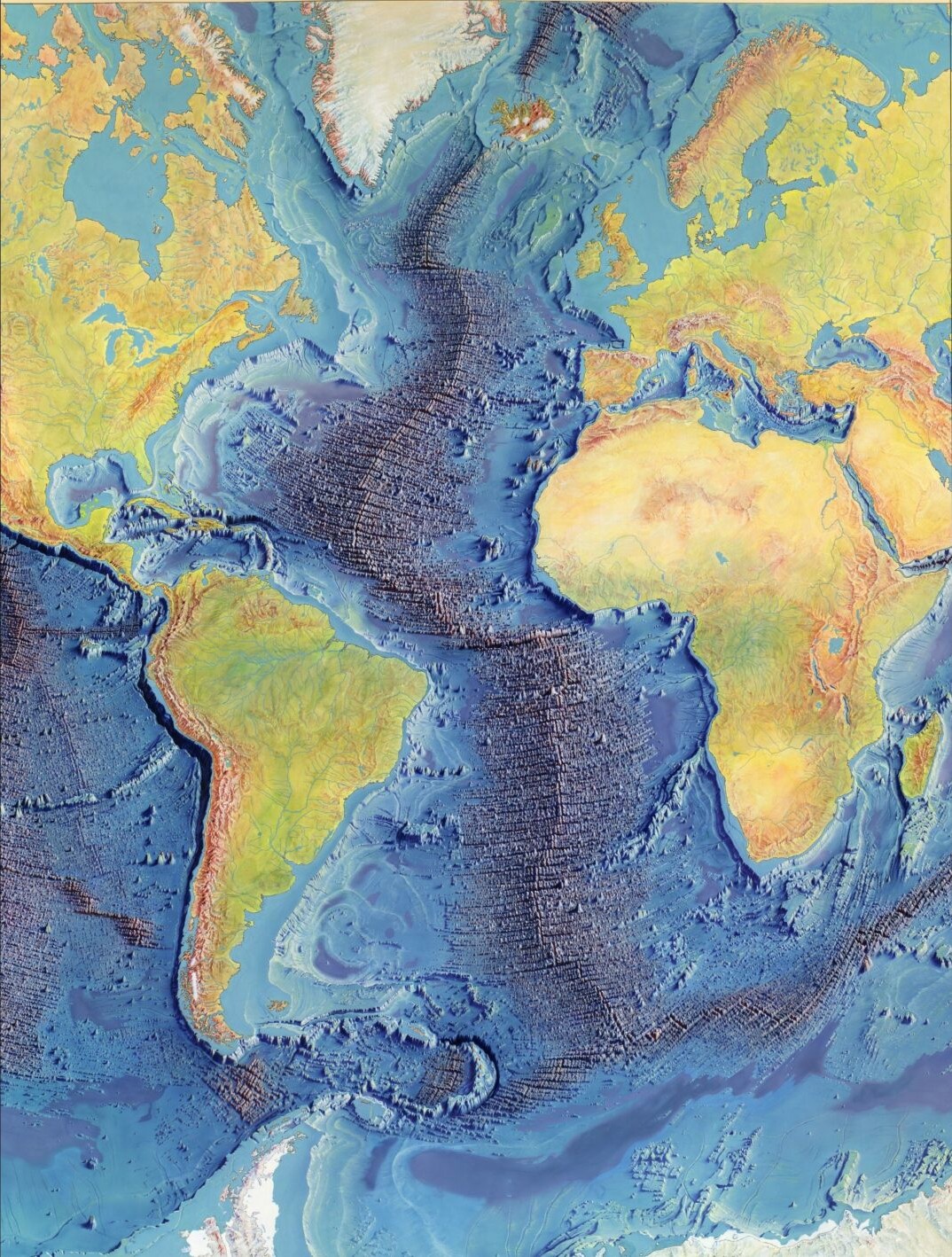
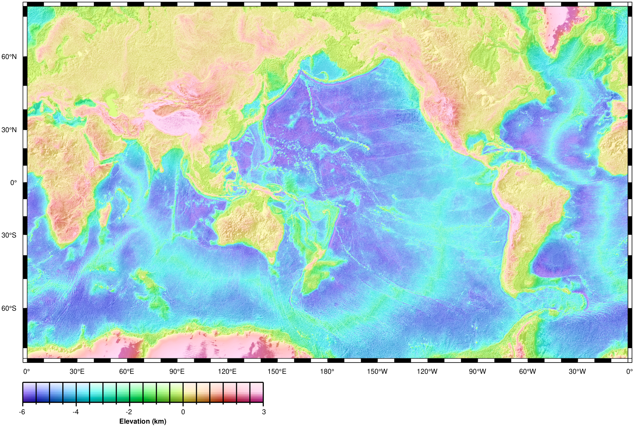
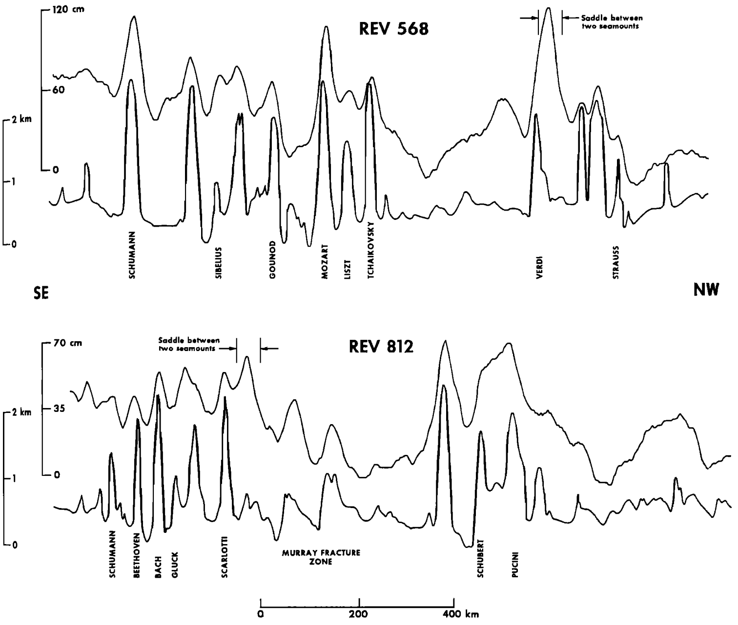
Bathymetric Prediction From SEASAT Altimeter Data (Dixon et al. 1983)
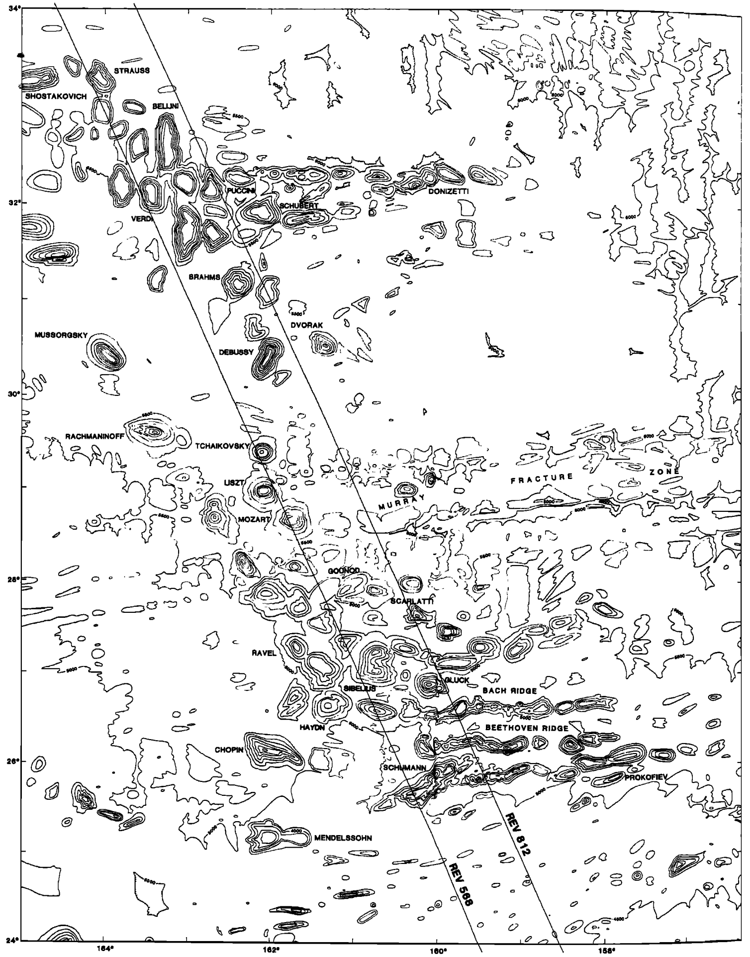
Bathymetric Prediction From SEASAT Altimeter Data (Dixon et al. 1983)
Gravitational potential
Gravitational potential is the the work (energy transferred) per unit mass that would be needed to move an object to that point from a distance infinitely far away. Recall that: $\mathrm{work = force~\times~displacement}$
The acceleration due to gravity is constant along an equipotential surface. How is the geoid related to gravitational potential?
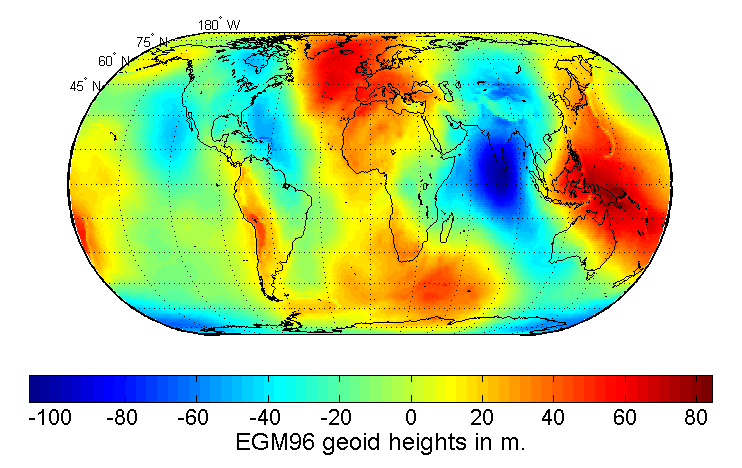
The geoid (a model) is the ocean surface elevation if winds and tides were absent.
If the Earth is isostatically compensated, why does the geoid (sea-surface) vary?
Strain in the asthenosphere removes any stress that exists due to force imbalances (ie density contrasts).. so geoid variations must:
- be small enough that the lithosphere can hold that stress
- be caused by other dynamic forces:
- convection/dynamic topography
- topography that changes faster than the asthenosphere can compensate (faster than the strain rate)
If the Earth is isostatically compensated, why does the geoid (sea-surface) vary?
- G=6.6743e-11 $\frac{m^3}{kg~s^2}$
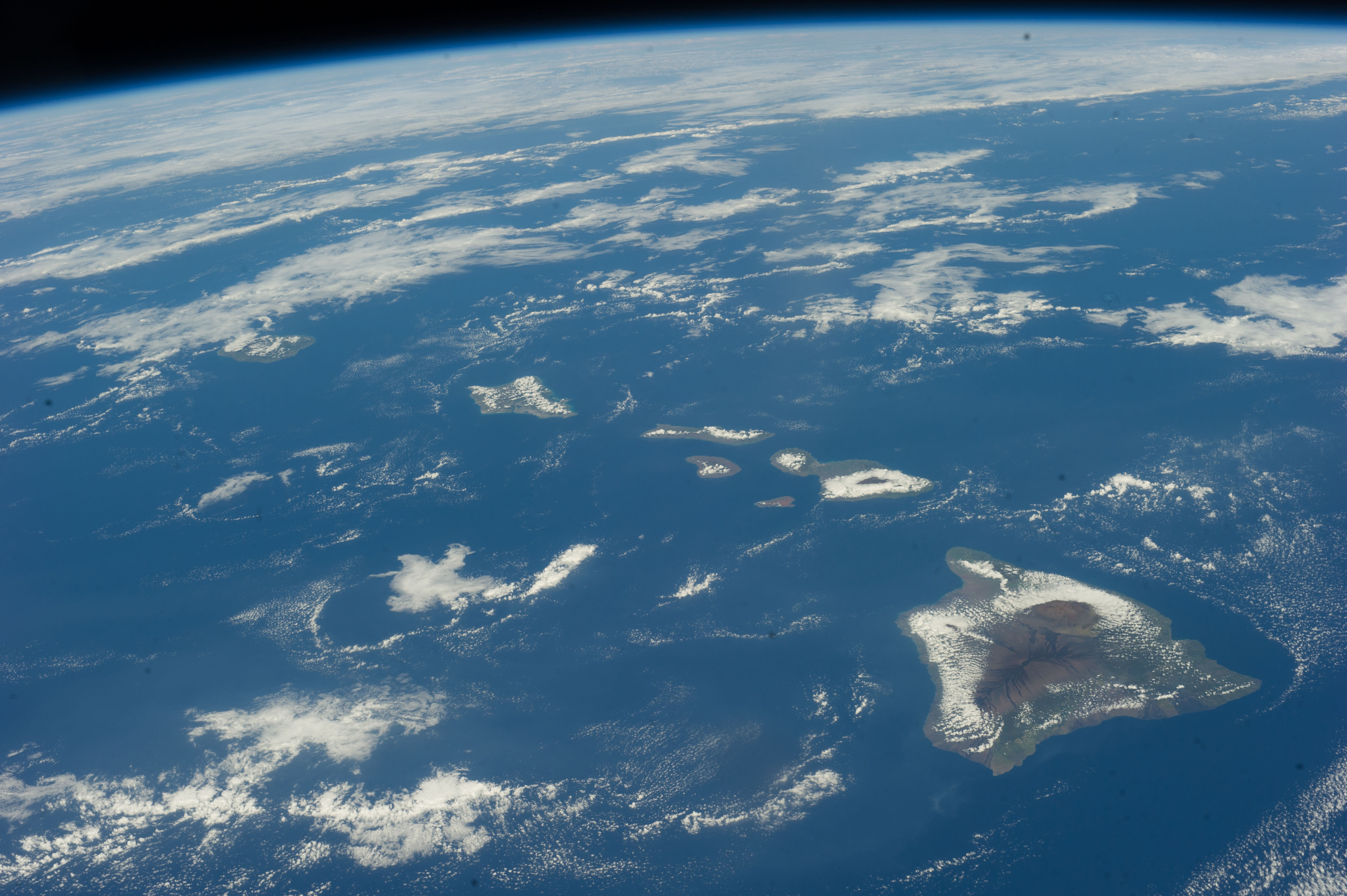
- Mass of the big island: 1.6e15 kg
- Mass of Earth: 5.97e24 kg
- Radius of Earth: 6.378e6 m
- Depth of seafloor: 6e3 m
Assume that the island is exactly 6 km tall. How is the acceleration due to gravity at sea level different above this island when compared to some far away location in the Pacific that has no island? Is it higher/lower? How much so?
If the Earth is isostatically compensated, why does the geoid (sea-surface) vary?
- G=6.6743e-11 $\frac{m^3}{kg~s^2}$
- Mass of the big island: 1.6e15 kg
- Mass of Earth: 5.97e24 kg
- Radius of Earth: 6.378e6 m
- Depth of seafloor: 6e3 m
Assume that the island is exactly 6 km tall. How is the acceleration due to gravity at sea level different above this island when compared to some far away location in the Pacific that has no island? Is it higher/lower? How much so? Now consider the force 3 km away from the island. What percent of the force is felt at this distance?
If the Earth is isostatically compensated, why does the geoid (sea-surface) vary?
- G=6.6743e-11 $\frac{m^3}{kg~s^2}$
- Mass of the big island: 1.6e15 kg
- Mass of Earth: 5.97e24 kg
- Radius of Earth: 6.378e6 m
- Depth of seafloor: 6e3 m
Assume that the island is exactly 6 km tall. How is the acceleration due to gravity at sea level different above this island when compared to some far away location in the Pacific that has no island? Is it higher/lower? How much so? Now consider the force 3 km away from the island. What percent of the force is felt at this distance? Repeat this same exercise using a point mass that is on the sea-floor (ie deeper than the previous calculation). The exact mass here doesn't matter. What percent of the force due to that mass is experienced 3 km away on the sea surface?
import numpy as np
from matplotlib import pyplot as plt
G=6.6743e-11# m3 kg-1 s-2
## point mass at 0,-6km
r2 = np.linspace(0,6)
mass = 1
f = G*mass/((r2**2+6**2)**(1/2))
plt.plot(r2,100*f/np.max(f),label='6km deep')
f = G*mass/((r2**2+3**2)**(1/2))
plt.plot(r2,100*f/np.max(f),label='3km deep')
f = G*mass/((r2**2+1**2)**(1/2))
plt.plot(r2,100*f/np.max(f),label='1km deep')
plt.legend(loc='lower left')
_=plt.gca().set_xlabel('Lateral distance from mass')
_=plt.gca().set_ylabel('% of force experienced')

If the Earth is isostatically compensated, why does the geoid (sea-surface) vary? (Summary)
- small amplitude differences in gravitational potential are maintained by lithosphere strength
- due to lateral differences in density (ie ocean at 3km next to basalt at 3km)
- low frequency (long wavelength) variations in gravitational potential are due to difference deeper in the Earth
- high frequency (short wavelength) variations are due to differences near the surface of the Earth
Mapping the sea-floor
- Altimetry data decomposed into high frequency (low wavelength) and low frequency (high wavelength) spectral components
- Low frequency components are combined with ship soundings to estimate deeper Earth density structures
- High frequency components are used to interpolate between soundings, assuming deep structure constant
- High frequency components are used to resolve very shallow density contrasts (such as sea-mounts)
Returning to the plate model and old oceanic lithosphere
Returning to the plate model and old oceanic lithosphere