Lecture 14 Carbonates and Age models
- Carbon cycle
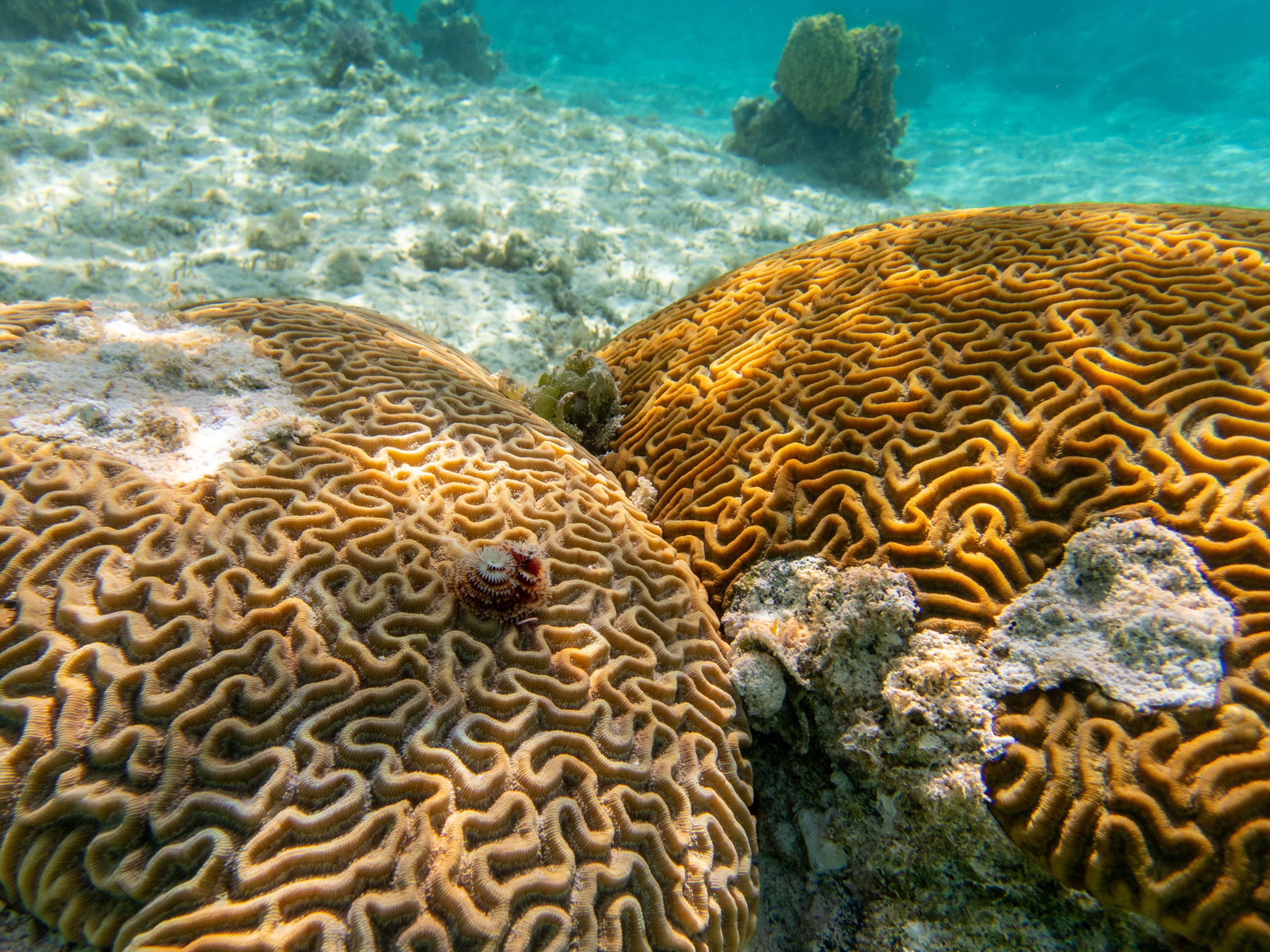
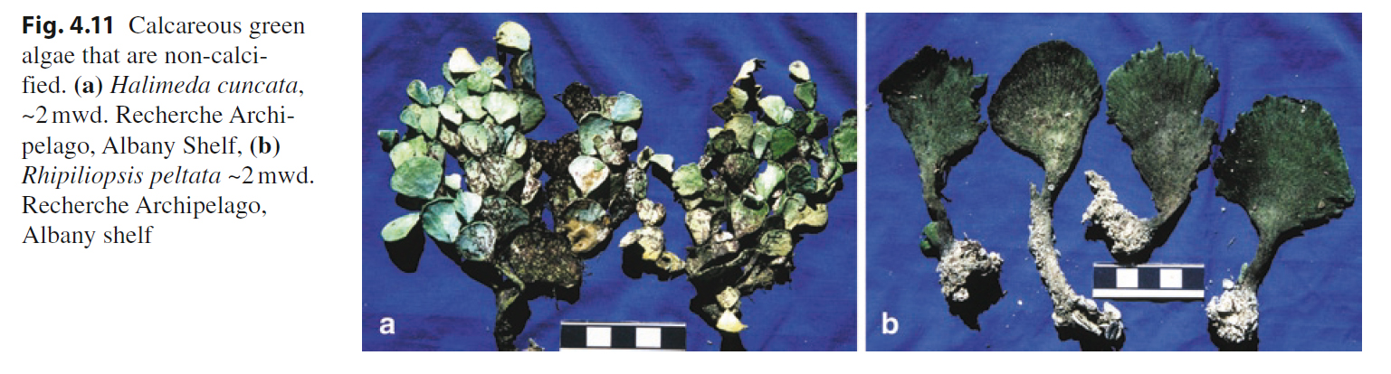
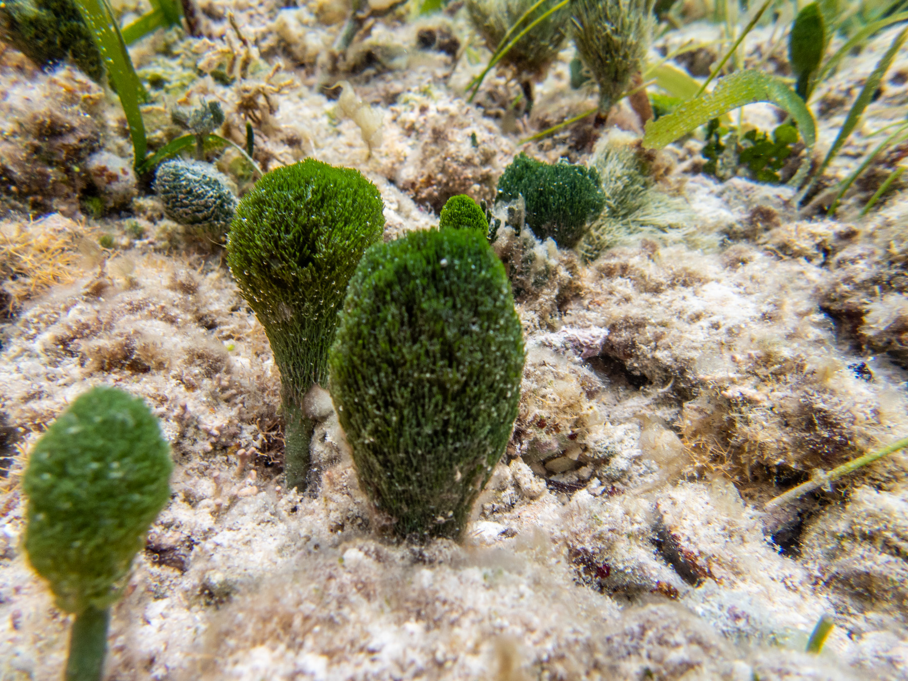
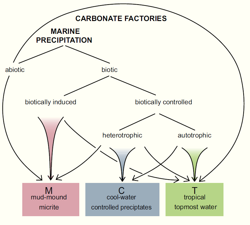
- Carbonate Factories
- T vs C vs M
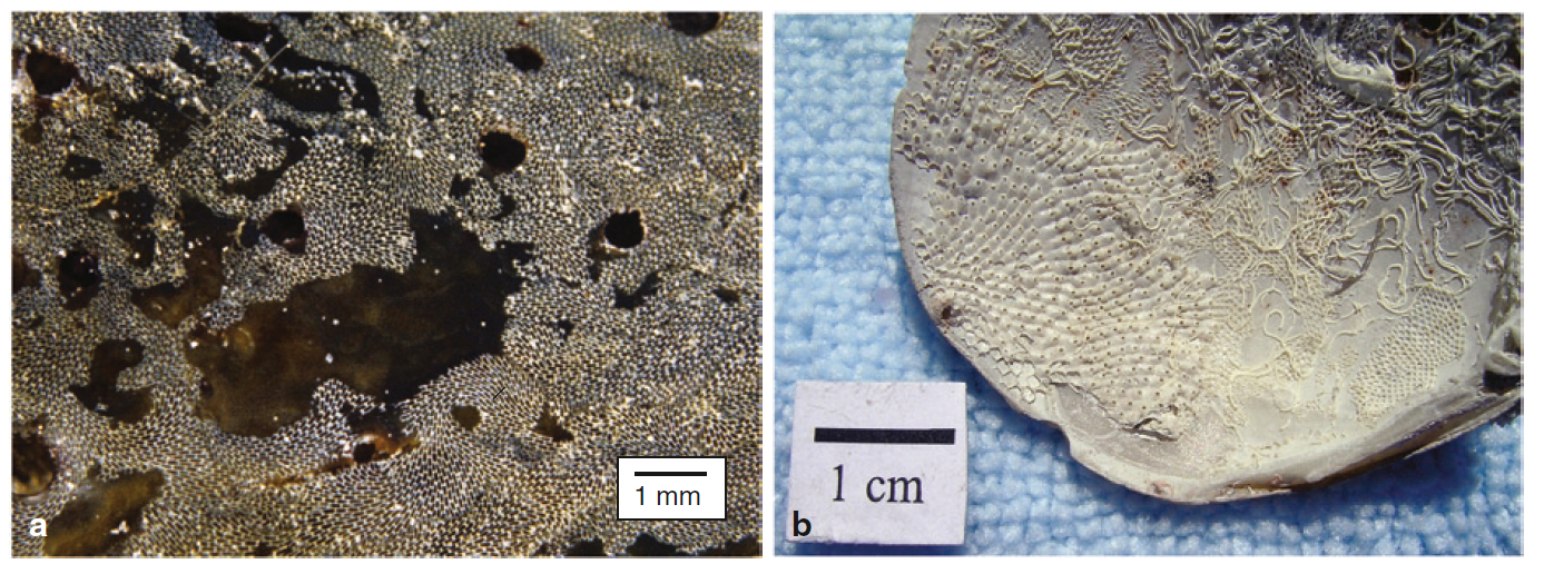
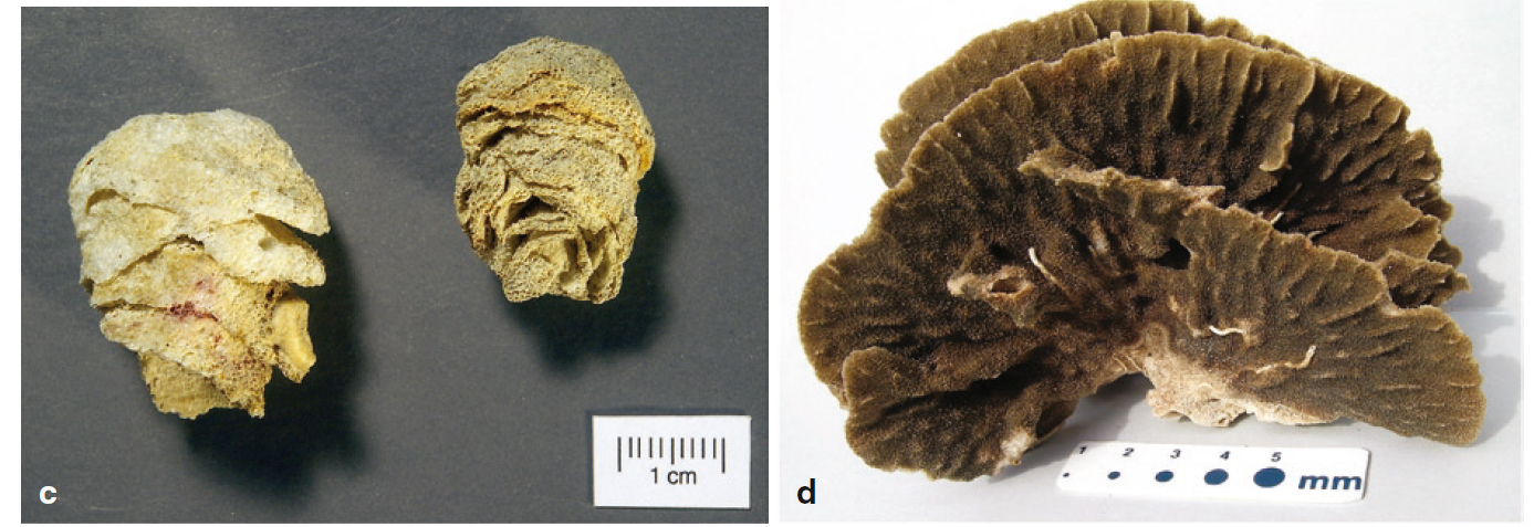
- Examples of each
- Sedimentation rates and growth potential of each
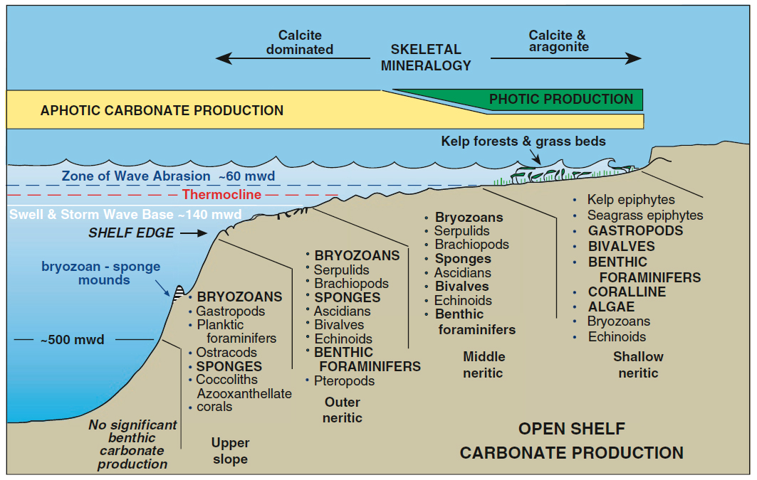
- Geometry of Carbonate Accumulations
- Modeling Carbonate Stratigraphy
- Carbonate Factories
- Age model implementations
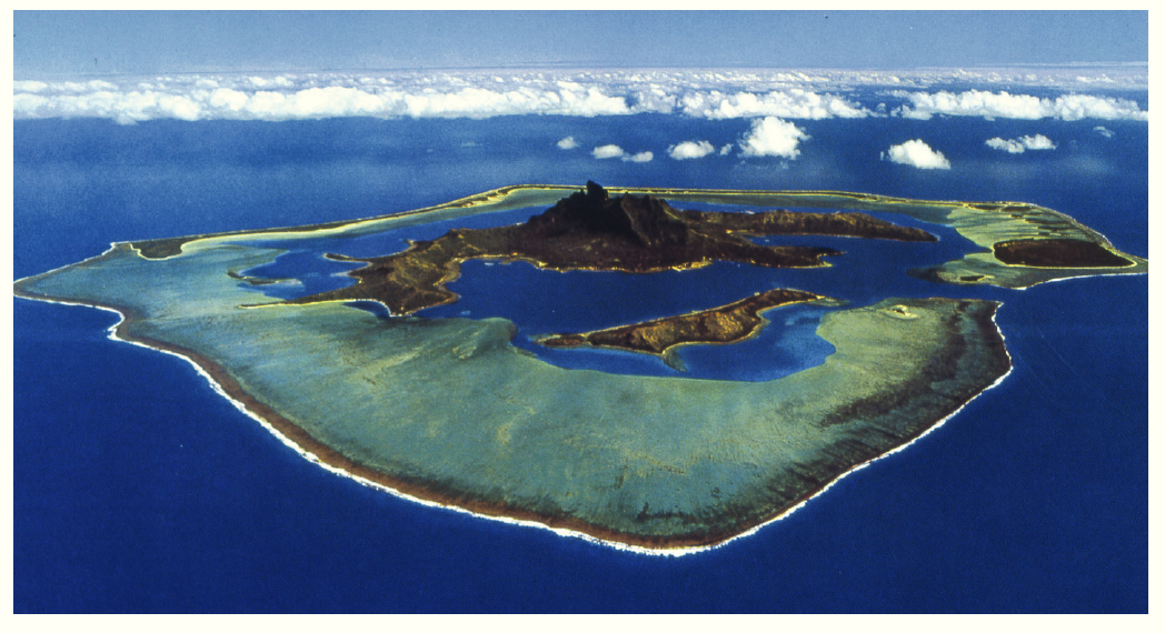
World Reef Map https://maps.lof.org/lof
Lets think a bit more about production rates..
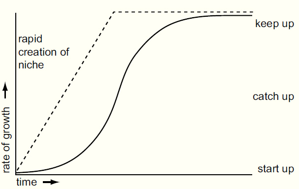
Lets think a bit more about production rates..
Lets think a bit more about production rates..
import numpy as np
from matplotlib import pyplot as plt
%matplotlib inline
dz = np.linspace(0,100,1000)
extinction_coeff = 0.2
light_z = np.exp(-extinction_coeff*dz)
plt.plot(light_z,-dz,label='light')
light_base=.1 #minimum light needed for full capacity
production_capacity = 1
production_z = production_capacity * np.tanh(light_z/light_base) #tanh gives the smoothing
plt.plot(production_z,-dz,label='carbonate production')
plt.gca().set_ylim([-40,0]); plt.legend(loc='best'); plt.gca().set_ylabel('depth (m)')
Text(0, 0.5, 'depth (m)')

def prod_func(z,light_base=0.1,extinction_coeff = 0.2):
    light_z = np.exp(-extinction_coeff*z)
    return np.tanh(light_z/light_base)
plt.plot([0,1000],[0,0],label='sea level')
dx = np.linspace(0,1000,1000)
topography = np.zeros(1000)-200
topography[dx>300]=-10
topography[dx>700]=-200
plt.plot(dx,topography,label='topography')
plt.gca().set_ylabel('depth (m)');plt.legend(loc='best',fontsize=10)
<matplotlib.legend.Legend at 0x7ff395e17760>

plt.plot(dx,prod_func(-topography),label='production\ncapacity')
plt.legend(loc='best',fontsize=10)
<matplotlib.legend.Legend at 0x7ff395c15610>

Now we need to decrease productivity in shallower/restricted water
For each grid point, we want some measure of how much nearby deep water there is..
## We will use a convolution for our implementation.. lets take a look at np.convolve
signal = np.sin(np.linspace(0,100,1000))
plt.plot(signal)
plt.plot(np.convolve(signal,signal[:10]))
[<matplotlib.lines.Line2D at 0x7ff3934d3730>]

from scipy.signal import gaussian
window_size = 50
standard_deviation = 10
plt.plot(gaussian(1+2*window_size,standard_deviation))
[<matplotlib.lines.Line2D at 0x7ff393750970>]

fig=plt.figure(figsize=(15,4))
plt.subplot(1,3,2)
restriction = np.convolve(topography,gaussian(1+2*window_size,standard_deviation),mode='valid')
restriction -= np.min(restriction)
restriction /= 7000 #scaling factor
plt.plot(dx[50:-50],restriction)
plt.gca().set_title('Production stress due to shallow/restricted water')
plt.subplot(1,3,1)
plt.plot(dx,topography,color='k')
plt.gca().set_title('topography')
plt.subplot(1,3,3)
productivity = prod_func(-topography)
plt.plot(dx,productivity,label='production\ncapacity')
productivity[window_size:-window_size]=productivity[window_size:-window_size]*(1-restriction)
plt.plot(dx,productivity,label='production\ncapacity\nrestriction')
plt.legend(loc='upper right',fontsize=10);

dt = 1  # timestep
base_level_rise = 100  # long term subsidence in meters
dx = 10  # x grid spacing
total_time = 3e6  # duration of simulation in years
initial_baselevel = 1  # in meters
sed_Q = 0.0  # sedimentation flux

#create an instance of Diffuse1D (defined above)
model = Diffuse1D(
    length=10000,
    spacing=dx,
    tstep=dt,
    left=0,
    right=0,
    K=2e-2,
    sed_Q=sed_Q,
    no_flux_boundary=True,
)

xt = np.linspace(0, total_time, 10000)  # creating uniform timegrid
RSL1 = -1.5 * np.sin(xt * 2 * np.pi * (1 / 20000))  # cyclic sea level component 1
RSL2 = 1 * sawtooth_wave(5, xt * 2 * np.pi * (1 / 100000))  # cyclic sea level component 2
RSL = (base_level_rise / (total_time) * xt + initial_baselevel)  # cyclic sea level + subsidence
# creates a function in the Diffuse1D model mapping your sea level boundary condition to time
model.set_baselevel(xt, RSL)
#to plot your model sea level boundary condition
plt.plot(xt/1000,model.base_level_fun(xt))
plt.gca().set_xlabel('Time (kilo-years)')
plt.gca().set_ylabel('Base level')
Text(0, 0.5, 'Base level')

plt.plot(model.u)
model.u=topography
plt.plot(model.u)
for i in tqdm(range(1000)):
    model.run_step()
plt.plot(model.u)

for i in tqdm(range(2000)):
    model.run_step()
plt.plot(model.u)
plt.gca().set_ylim([-50,0])
0%| | 0/1000 [00:00<?, ?it/s]
0%| | 0/2000 [00:00<?, ?it/s]
(-50.0, 0.0)

dt = 10  # timestep
base_level_rise = 60  # long term subsidence in meters
dx = 10  # x grid spacing
total_time = 1e6  # duration of simulation in years
initial_baselevel = 1  # in meters
sed_Q = 0.0  # sedimentation flux

#create an instance of Diffuse1D (defined above)
model = Diffuse1D(
    length=10000,
    spacing=dx,
    tstep=dt,
    left=0,
    right=0,
    K=2e-2,
    sed_Q=sed_Q,
    no_flux_boundary=True,
)

xt = np.linspace(0, total_time, 10000)  # creating uniform timegrid
RSL1 = 2 * np.sin(xt * 2 * np.pi * (1 / 1e5))  # cyclic sea level component 1
RSL = (base_level_rise / (total_time) * xt + initial_baselevel +RSL1)  # cyclic sea level + subsidence
# creates a function in the Diffuse1D model mapping your sea level boundary condition to time
model.set_baselevel(xt, RSL)
model.u=topography
model.carb_rate = .0015
#to plot your model sea level boundary condition
plt.plot(xt/1000,model.base_level_fun(xt))
plt.gca().set_xlabel('Time (kilo-years)')
plt.gca().set_ylabel('Base level')
Text(0, 0.5, 'Base level')

# initial lists to store model outputs throughout the simulation
beds = [] #model topography
age = [] #model time
rsl = [] #relative (local) sea level
sed_on = True
progress_bar = tqdm(range(int(total_time / dt / 1))) #run the model for the full duration, the tqdm wrapper provides a progress bar
for i in progress_bar:
    model.run_step() #run 1 timestep dt
    if i%50==0: #save every 50 steps to our lists
        beds.append(model.u)
        age.append(model.time)
        rsl.append(model.base_level)
0%| | 0/100000 [00:00<?, ?it/s]
skip=25
animate_beds(beds=beds[::skip],otime=age[::skip],rsl=rsl[::skip],aspect=2, ymin=-20, ymax=75, color=True)

column_number = 325
bed_facies, bed_bottom, bed_thickness, bed_colors = get_strat_column(beds, age, rsl, column_number, skip=10)
plot_column(bed_facies, bed_bottom, bed_thickness, bed_colors, left=column_number)
plt.gca().set_aspect(.05)

 column_number = 500
bed_facies, bed_bottom, bed_thickness, bed_colors = get_strat_column(beds, age, rsl, column_number, skip=10)
plot_column(bed_facies, bed_bottom, bed_thickness, bed_colors, left=column_number)
plt.gca().set_aspect(.05)

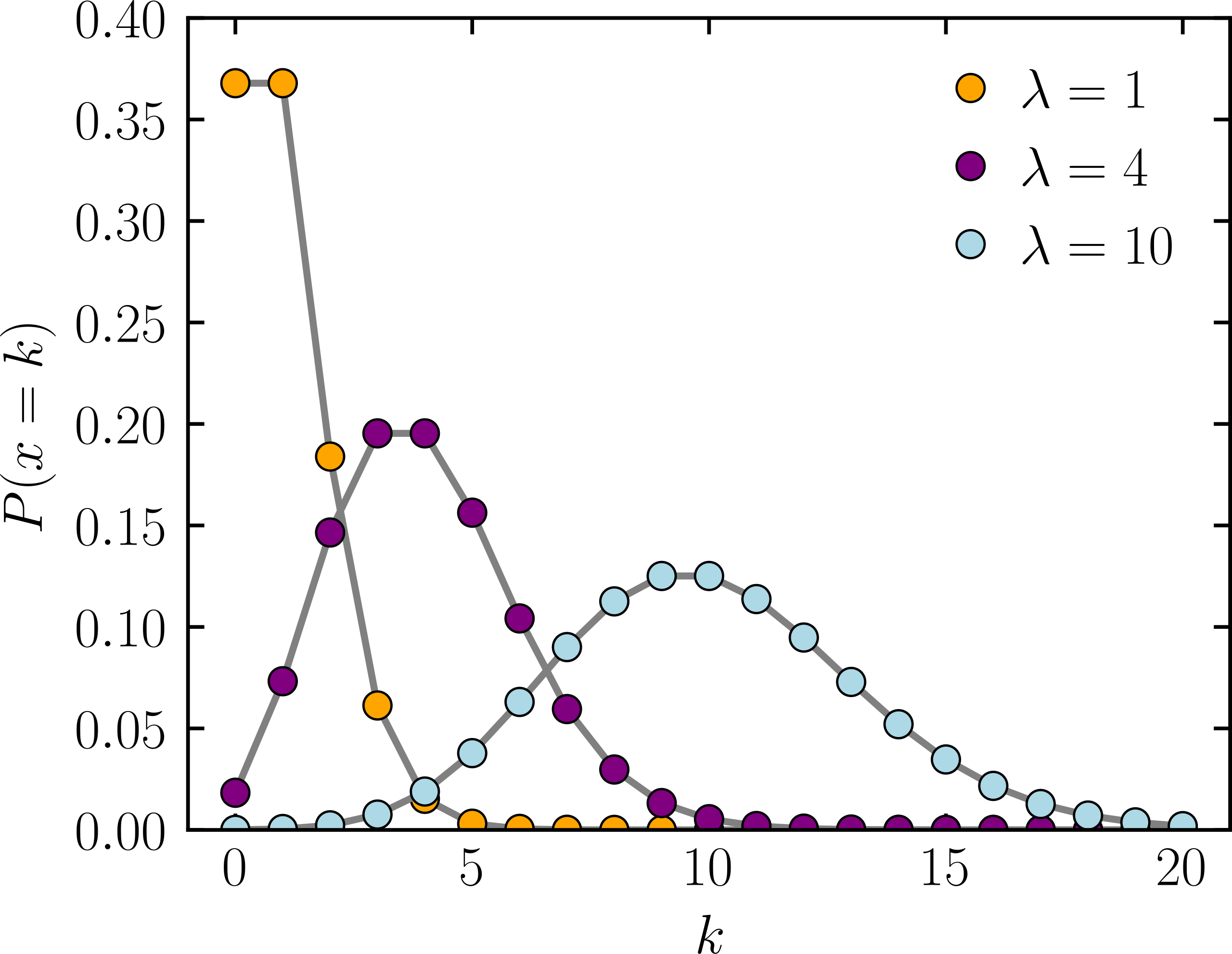
Poisson-Gamma Age Models
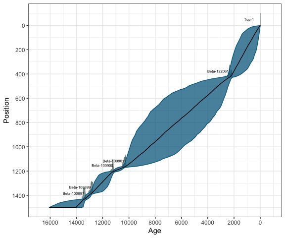
Poisson distribution is a discrete probability distribution that expresses the probability of a given number of events occurring in a fixed interval of time or space if these events occur with a known constant mean rate $\lambda$ and are independent of the time since the last event.
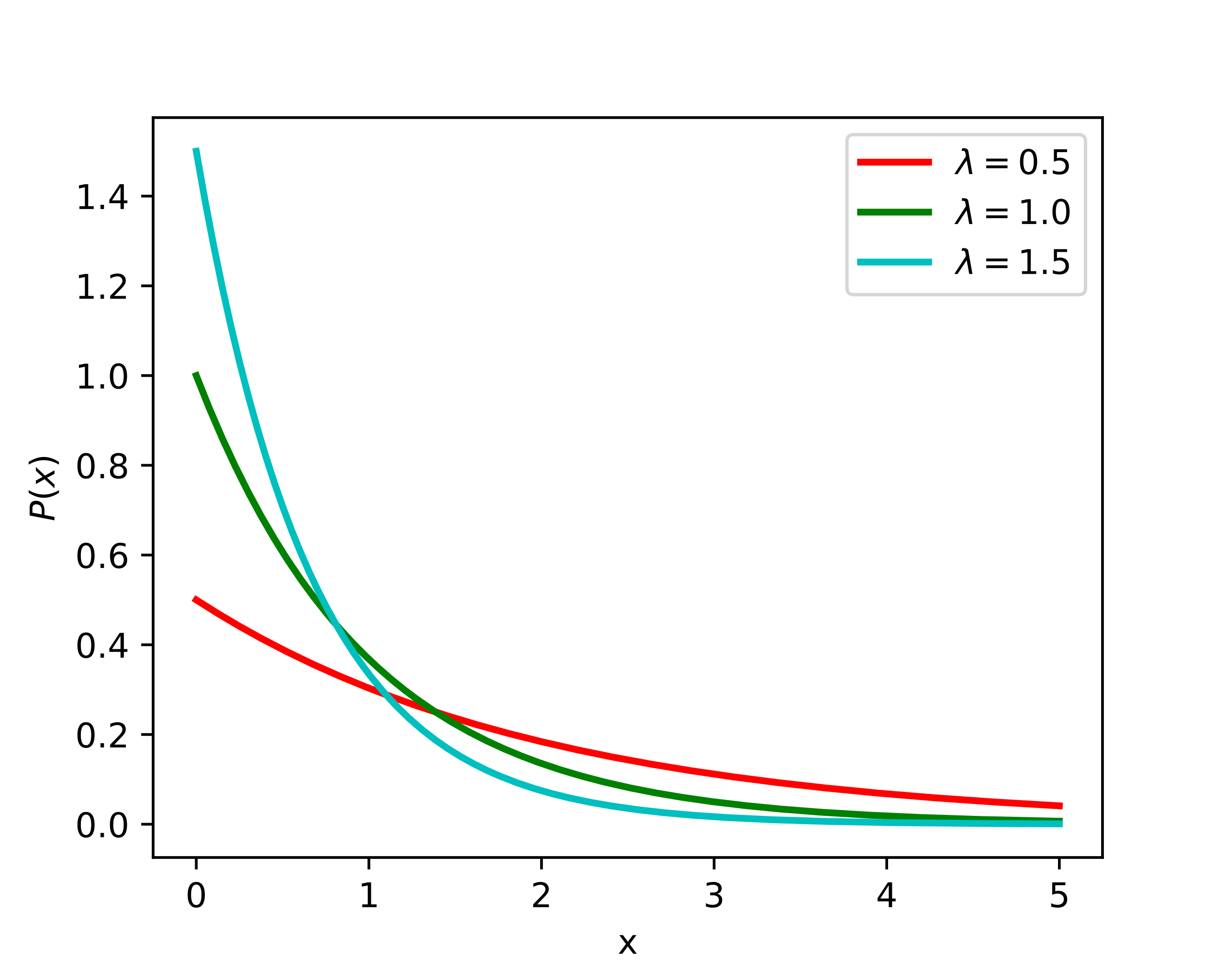
Exponential distribution (a particular case of the of gamma distribution) is the probability distribution of the time between events in a Poisson point process
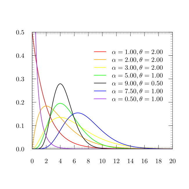
Gamma distribution if $\alpha$ is a positive integer is the sum of $\alpha$ independant exponentially distributed random variables with a mean of $\theta$.
Let's do a simple trial to check our intuition..
import numpy as np
from matplotlib import pyplot as plt
import seaborn as sns
fig=plt.figure(figsize=(5,5))
a = np.random.uniform(0,1,100000)
b = a<0.1  ## 10 percent of the time
sns.kdeplot(np.diff(np.where(b)[0]),color=sns.color_palette('deep')[2],fill=True,lw=3) #time-lags
# c = np.random.exponential(10,100000) ## duration between events when average (lambda) is 10
# sns.kdeplot(c,color=sns.color_palette('deep')[1],fill=True,lw=3)
sns.despine()

Deciding on number of sedimentation rate changes
plt.plot([0,1],[0,1],'s-')
plt.gca().set_xlabel('time')
plt.gca().set_ylabel('height')
for i in range(10):
    pts=np.random.poisson(10) #discrete number of changes
    if pts>0:
        h_gaps=np.cumsum(np.random.gamma(1,1, pts))
        h_gaps=h_gaps/np.max(h_gaps)
        t_gaps=np.cumsum(np.random.gamma(1,1, pts))
        t_gaps=t_gaps/np.max(t_gaps)
        plt.plot([0,*t_gaps],[0,*h_gaps],'s-')

What do the parameters of the gamma function do?
from scipy import stats
fig=plt.figure(1, figsize=(12,6)); ax=fig.add_subplot(111)
g_shape=1.5; g_loc=0; g_scale=1
gam_hist=np.random.gamma(g_shape,g_scale, 10000) #10K draws with shape = 1.5 and scale = 1
x=np.linspace(0,max(gam_hist),1000)
gam=stats.gamma.pdf(x,g_shape,g_loc,g_scale) #continuous function
ax.hist(gam_hist,density=True,alpha=0.75,color='#6495ED',
        label=r'$\lambda$ = %2.1f; $\mu$ = %2.3f' % (g_shape*g_scale,np.mean(gam_hist))); ax.plot(x,gam,'k--')
g_shape=10.5; g_loc=0; g_scale=1 #10K draws with shape = 10.5 and scale = 1
gam_hist=np.random.gamma(g_shape,g_scale, 10000)
x=np.linspace(0,max(gam_hist),1000); gam=stats.gamma.pdf(x,g_shape,g_loc,g_scale) #continuous function
ax.hist(gam_hist,density=True,alpha=0.75,color='#B22222',
        label=r'$\lambda$ = %2.1f; $\mu$ = %2.3f' % (g_shape*g_scale,np.mean(gam_hist))); ax.plot(x,gam,'k--')
#plot labels
ax.set_title('examples of gamma distributions')
ax.legend(); _=ax.text(0.99,0.725,', '.join(['%2.3f' %(g) for g in gam_hist[0:6].tolist()]) + ', ... ',
                       transform=ax.transAxes,horizontalalignment='right',fontsize=15)

gamma distributions in sedimentology
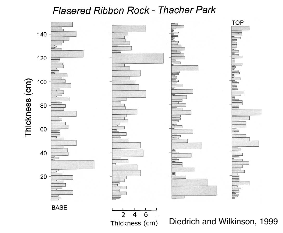
gamma distributions in sedimentology
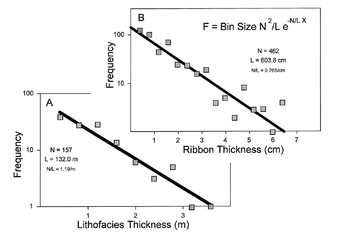
gamma distributions in sedimentology
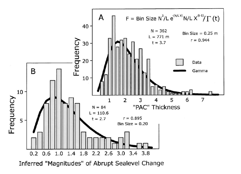
Appendix: more on gamma distributions in sedimentology
#timesteps; probability of change; starting state
t=20000; prob=0.25; state=1
#minimum beds in a parasequence
min_couplet_num=3

#switch state
sed=np.array([state*-1 if np.random.random()<prob else state for i in range(t)])
#find the "on" periods
on=np.where(sed==1)[0]

#find indices of consecutive "on" periods
on_breaks=list(np.where(np.diff(on)!=1)[0]+1)

#group into pairs
on_breaks=[0]+on_breaks+[len(on)]
on_breaks=list(zip(on_breaks[0:-1],on_breaks[1:]))

#calculate lengths of "sediment on" period
on_time=[]
for o in on_breaks:
    on_time.append(len(on[o[0]:o[1]]))

#here, the "on" periods are used to bundle couplets
#--> value = number of couplets
on_time=np.cumsum(np.array(on_time)+min_couplet_num-1)
couplet_idx=list(zip(list(on_time[0:-1]),list(on_time[1:])))
couplet_idx=[tuple((0, couplet_idx[0][0]))]+couplet_idx
#generate thickess of those couplets
couplets=np.random.gamma(1,1, couplet_idx[-1][1])
#package them up
bundles=[np.sum(couplets[i[0]:i[1]]) for i in couplet_idx]
Appendix: more on gamma distributions in sedimentology
#first hundred couplets for plotting
demo_couplets=list(np.cumsum(couplets)[0:100])
demo_couplets=[0]+demo_couplets
demo_couplets=list(zip(demo_couplets[0:-1],demo_couplets[1:]))
#make thickness vs. height boxes
couplet_boxes=[]
for d in demo_couplets:
    xy=np.array([(0,d[0]),(d[1]-d[0],d[0]),(d[1]-d[0],d[1]),(0,d[1])])
    rect = Polygon(xy,closed=True,facecolor="#"+''.join([np.random.choice([a for a in '0123456789ABCDEF']) for j in range(6)]))
    couplet_boxes.append(rect)
#bundles of couplets
demo_bundles=np.cumsum(bundles)[0:100]
demo_bundles=demo_bundles[demo_bundles<demo_couplets[-1][1]]
Appendix: more on gamma distributions in sedimentology
fig=plt.figure(1,figsize=(20,11)); ax=fig.add_subplot(121); ax.plot(sed[0:100],range(100)) #plot sedimentation history
ax.set_ylabel('time'); ax.set_xlabel('sediment switch'); ax.set_xticks([-1.0,1.0]); ax.set_xticklabels(['off','on'])
ax=fig.add_subplot(122); _=[ax.add_patch(r) for r in couplet_boxes] #plot bed thickness vs. height
ax.set_xlim([0,np.ceil(max(couplets[0:100]))]); ax.set_ylim([0,np.ceil(demo_couplets[-1][1])])
ax.set_ylabel('height (meters)');ax.set_xlabel('bed thickness (meters)')
_=[ax.plot(ax.get_xlim(),[d,d],'k--') for d in demo_bundles] #plot the parasequence boundaries
_=ax.text(ax.get_xlim()[1],demo_bundles[0],'parasequence top',horizontalalignment='right',verticalalignment='bottom',fontsize=15)

Appendix: more on gamma distributions in sedimentology
#histogram of bed thickness
fig=plt.figure(1,figsize=(20,11)); ax=fig.add_subplot(221)
ax.hist(couplets,bins=30,density=True); ax.set_xlabel('bed thickness (meters)')
#histogram of number of beds in a parasequence
ax=fig.add_subplot(222); ax.hist([i[1]-i[0] for i in couplet_idx],bins=30,density=True); ax.set_xlabel('beds per parasequence')
#histogram of parasequence thickness
ax=fig.add_subplot(212); ax.hist(bundles,bins=30,density=True);_=ax.set_xlabel('parasequence thickness (meters)')
