Lectures 4-5: Modeling Bulk Transport (numerically)

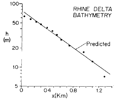
1. Kenyon and Turcotte (1985)
   1. Diffusion as a transport mechanism
2. A more powerful diffusive model
   1. Live example with variable sea level
   2. Solving the diffusion equation numerically
      1. The derivative function
      2. Finite difference methods
   3. An explicit solution to the diffusion equation
      1. Stability
   4. An implicit solution to the diffusion equation

We acknowledge and respect the lək̓ʷəŋən peoples on whose traditional territory the university stands and the Songhees, Esquimalt and W̱SÁNEĆ peoples whose historical relationships with the land continue to this day.

Kenyon and Turcotte (1985): Diffusion

K&T to convince you that diffusion, or bulk sediment transport, is a reasonable approximation

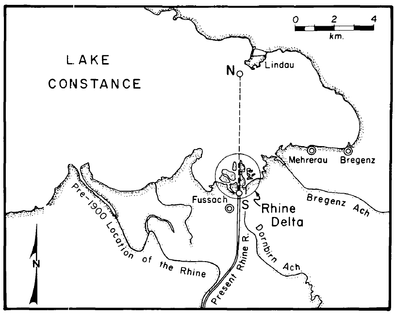
Diffusion as a transport mechanism

When we assume that diffusive transport exerts an important control on landscape dynamics we generally accept that particles on the surface of the planet are in constant complex motion, and there is some downslope bias introduced by gravity to those motions. Over time, diffusion can be assumed to smooth topography (by the transport of material downslope).

$$\begin{equation} \dfrac{\partial h}{\partial t} = K \dfrac{\partial^2 h}{\partial x^2}\tag{hillslope application} \end{equation}$$

A more powerful diffusion model

Over the next few weeks in your assignments you will be building a 1-D diffusive transport model to explore how variations in the following properties change the stratigraphic architecture of a basin:

1. transport
2. sediment supply
3. accomodation space

An example: varying accomodation space

x_ran = np.linspace(0,total_time,len(pbar))
fig=plt.figure(figsize=(15,10))
plt.plot(x_ran,model.base_level_fun(x_ran), lw=3)
plt.gca().set_xlabel('Time (years)')
plt.gca().set_ylabel('Base level')

Text(0, 0.5, 'Base level')

animate_beds(beds=beds,otime=otime,rsl=rsl,aspect=5, ymin=-100)

fig=plt_strat()

Solving the diffusion equation numerically

We can use the diffusion equation to simulate more complicated transport than the specific case from Kenyon and Turcott 1985. Generally, after defining a few properties of the system (What properties?) we can solve how that system will change over time. However, there is no exact, or analytical form to this solution -- we must solve the equation by numerical approximation.

$$\begin{equation} \dfrac{\partial h}{\partial t} = K \dfrac{\partial^2 h}{\partial x^2} \end{equation}$$

(initial topography, boundary conditions at the edges)

The Derivative Function

Recall: what is the definition of the derivative function $f'(x)$?

$$ \begin{equation} f'(x) = \lim_{\Delta x\to0} \dfrac{f(x+\Delta x)-f(x)}{\Delta x} \end{equation} = \dfrac{\Delta f}{\Delta x} $$

While we can't calculate $\Delta x$ and $\Delta f$ for $\lim{(\Delta x\to0)}$ CPUs have no trouble calculating $\dfrac{\Delta f}{\Delta x}$ for a sufficiently small value of $\Delta x$

Finite difference methods

In fact, we have many possible approaches to estimating derivatives using sufficiently small values of $\Delta x$, and these methods are collectively known as finite difference methods. These methods make use of Taylor's theorem:

$\begin{equation} f(x + \Delta x) = f(x) + \dfrac{f'(x)}{1!}(\Delta x) + \dfrac{f''(x)}{2!}(\Delta x)^2 + ... \end{equation} \label{eq:taylor}\tag{Taylor series} $

What happens to the size of each higher order term in the series?

We describe the error of an approximation by the degree of the term where the series is truncated. First order: $O(\Delta x)$, second order: $O(\Delta x^2)$, third order: $O(\Delta x^3)$, etc...

$$ \begin{equation} f(x + \Delta x) \color{red}{\approx} f(x) + \dfrac{f'(x)}{1!}(\Delta x) \color{Gray}{+ \dfrac{f''(x)}{2!}(\Delta x)^2 + ...} \end{equation} $$

The forward-difference approximation of the first derivative with error $O(\Delta x)$:

$$ \begin{equation} f'(x) = \dfrac{f(x+\Delta x)-f(x)}{\Delta x} \end{equation} $$

Any guesses to what the backward-difference looks like?

$$ \begin{equation} f'(x) = \dfrac{f(x) - f(x-\Delta x)}{\Delta x} \end{equation} $$

For this next part, it helps to consider a more specific case where we know our function $f(x)$ for values of $x$ separated by $\Delta x$. Let's call our function $h(x)$ for height or topography. (Draw cartoon of topography at a single timestep)

General		Specific
$$\begin{equation} f(x + \Delta x) = f(x) + \dfrac{\color{Blue}{f'(x)}}{1!}(\Delta x) + \dfrac{\color{Blue}{f''(x)}}{2!}(\Delta x)^2 + ... \end{equation} $$$$\begin{equation} f(x \color{red}{-} \Delta x) = f(x) + \dfrac{\color{Blue}{f'(x)}}{1!}(\color{red}{-}\Delta x) + \dfrac{\color{Blue}{f''(x)}}{2!}(\color{red}{-}\Delta x)^2 + ... \end{equation} $$		$$\begin{equation} right = center + \color{Blue}{h'(x)}\Delta x + \dfrac{\color{Blue}{h''(x)}}{2}\Delta x^2 \end{equation} $$$$\begin{equation} left = center \color{red}{-} \color{Blue}{h'(x)}\Delta x + \dfrac{\color{Blue}{h''(x)}}{2}\Delta x^2 \end{equation} $$

Using these two second-order truncations of the Taylor series, derive approximations for both of the unknowns (first and second derivative)

$$\begin{equation} \color{blue}{h''(x_i)} \approx \dfrac{\mathrm{left} - 2~\mathrm{center} + \mathrm{right}}{\Delta x^2} \tag{central-difference $\frac{\partial^2 h}{\partial x^2}$} \end{equation} $$$$\begin{equation} \color{blue}{h'(x_i)} \approx \dfrac{\mathrm{right}-\mathrm{left}}{2\Delta x} \tag{central-difference $\frac{\partial h}{\partial x}$} \end{equation} $$

Explicit solution

All this algebra leads us to an explicit solution to the diffusion equation: $$\begin{equation} \dfrac{\partial h}{\partial t} = K \color{blue}{\dfrac{\partial^2 h}{\partial x^2}} \end{equation}$$

$$\begin{equation} \dfrac{\partial h}{\partial t} \color{red}{\approx} K \color{blue}{\dfrac{\mathrm{left} - 2~\mathrm{center} + \mathrm{right}}{\Delta x^2}} \end{equation}$$

How do we handle $\dfrac{\partial h}{\partial t}$?

Let's look at a space-time grid for the problem..

Since we want to solve for the future timestep, we need to use an approximation for $\dfrac{\partial h}{\partial t}$ that includes the current time-step (known) and the future time-step (unknown). We will use the forward difference approximation for time:

General		Specific
$$ \begin{equation} f'(x) \approx \dfrac{f(x+\Delta x)-f(x)}{\Delta x} \end{equation} $$		$$\begin{equation} \dfrac{\partial h}{\partial t} \approx \dfrac{future-now} {\Delta t} \end{equation} $$

$$\begin{equation} \dfrac{\partial h}{\partial t} \color{red}{\approx} K \dfrac{\mathrm{left} - 2~\mathrm{center} + \mathrm{right}}{\Delta x^2} \end{equation}$$$$\begin{equation} \dfrac{\mathrm{\color{Blue}{future}-now}} {\Delta t} \color{red}{\approx} K \dfrac{\mathrm{left} - 2~\mathrm{center} + \mathrm{right}}{\Delta x^2} \end{equation}$$

$$\begin{equation} \dfrac{\mathrm{\color{Blue}{future}-now}} {1} \color{red}{\approx} \dfrac{K\Delta t}{\Delta x^2} \dfrac{\mathrm{left} - 2~\mathrm{center} + \mathrm{right}}{1} \end{equation}$$

Let $r=\dfrac{K\Delta t}{\Delta x^2}$

$$\begin{equation} \mathrm{\color{Blue}{future}} \color{red}{\approx} r \left(\mathrm{left} - 2~\mathrm{center} + \mathrm{right}\right) + \mathrm{now} \end{equation}$$

Recall: what is meant by the word $\mathrm{now}$ in this equation?

$$\mathrm{now = center}$$

$$ \begin{equation} \mathrm{\color{Blue}{future}} \color{red}{\approx} r~\mathrm{left} - 2~r~\mathrm{center} + r~\mathrm{right} + \mathrm{center} \end{equation} $$$$ \begin{equation} \mathrm{\color{Blue}{future}} \color{red}{\approx} r~\mathrm{left} + (1 - 2~r)~\mathrm{center} + r~\mathrm{right} \end{equation} $$$$ \begin{equation} \color{Blue}{h(x_i^{t+\Delta t}}) \color{red}{\approx} r~h(x_{i-\Delta x}) + (1 - 2~r)~h(x_{i}) + r~h(x_{i+\Delta x}) \end{equation} $$

$$ \begin{equation} \color{Blue}{h(x_i^{t+\Delta t}}) \color{red}{\approx} r~h(x_{i-\Delta x}) + (1 - 2~r)~h(x_{i}) + r~h(x_{i+\Delta x}) \end{equation} $$

We now have a separate equation for each point on our grid of interest $h(x_0)$ to $h(x_N)$ (with $h(x_i)$ above). How does the equation need to change at the boundaries $h(x_0)$ and $h(x_N)$?

$$ \begin{equation} \color{Blue}{h(x_0^{t+\Delta t}}) \color{red}{\approx} \end{equation} $$$$ \begin{equation} \color{Blue}{h(x_N^{t+\Delta t}}) \color{red}{\approx} \end{equation} $$

$$ \begin{equation} \color{Blue}{h(x_0^{t+\Delta t}}) \color{red}{\approx} r~(\mathrm{left~boundary~condition}) + (1 - 2~r)~h(x_{i}) + r~h(x_{i+\Delta x}) \end{equation} $$$$ \begin{equation} \color{Blue}{h(x_N^{t+\Delta t}}) \color{red}{\approx} r~h(x_{i-\Delta x}) + (1 - 2~r)~h(x_{i}) + r~(\mathrm{right~boundary~condition}) \end{equation} $$

Linear Algebra Refresher

We will use linear algebra to solve the system of equations (one equation per finite element $h_i$ in our model). There are two rules about matrix and vector operations that you will need to recall:

First, lets set: $ \begin{equation} B = \begin{bmatrix} b_{11}& b_{12}& b_{13}\\ b_{21}& b_{22}& b_{23}\\ b_{31}& b_{32}& b_{33}\\ \end{bmatrix} \end{equation} $ and $ \begin{equation} h = \begin{bmatrix} h_{0}\\ h_{i}\\ h_{n}\\ \end{bmatrix} \end{equation} $

What is $B$ multiplied by $h$?

The multiplication of matrix $B$ times vector $h$ produces a linear combination of the columns of the matrix where column $i$ is paired with the item $i$ in the vector $h$.

$$ \begin{equation} Bh= h_0 \begin{bmatrix} b_{11}\\ b_{21}\\ b_{31}\\ \end{bmatrix} + h_i \begin{bmatrix} b_{12}\\ b_{22}\\ b_{32}\\ \end{bmatrix} + h_N \begin{bmatrix} b_{13}\\ b_{23}\\ b_{33}\\ \end{bmatrix} \end{equation} $$

$$ \begin{equation} B = \begin{bmatrix} b_{11}& b_{12}& b_{13}\\ b_{21}& b_{22}& b_{23}\\ b_{31}& b_{32}& b_{33}\\ \end{bmatrix} \end{equation} $$

For our second rule, what is $B^{-1}B$ equal to?

By definition, the inverse matrix $B^{-1}$ undoes the effects of matrix $B$. $$ \begin{equation} B^{-1}B = \begin{bmatrix} 1& 0& 0\\ 0& 1& 0\\ 0& 0& 1\\ \end{bmatrix} \end{equation} $$

Note that the order from left to right is important when using the inverse matrix to solve systems of equations. For example, assuming that each of the following letters is a matrix, to solve for $X$ in $ABCXD=E$ we must multiply both sides of the equation by $D^{-1}$ on the right side, and then by $A^{-1}$, $B^{-1}$, $C^{-1}$ (in that order) on the left: $X=C^{-1}B^{-1}A^{-1}ED^{-1}$

Let's return to our approximation of the diffusion equation: $$ \begin{equation} \color{Blue}{h(x_i^{t+\Delta t}}) \color{red}{\approx} r~h(x_{i-\Delta x}) + (1 - 2~r)~h(x_{i}) + r~h(x_{i+\Delta x}) \end{equation} $$

Working in small groups spend the next X minutes converting the equation above into matrix form:

$$ \begin{equation} \begin{bmatrix} \color{blue}{h_0^{t+\Delta t} }\\ \color{blue}{h_i^{t+\Delta t}} \\ \color{blue}{h_N^{t+\Delta t}} \\ \end{bmatrix} = ???? \end{equation} $$

Our approximation of the diffusion equation in matrix form:

$$ \begin{equation} \begin{bmatrix} \color{blue}{h_0^{t+\Delta t} }\\ \color{blue}{h_i^{t+\Delta t}} \\ \color{blue}{h_N^{t+\Delta t}} \\ \end{bmatrix} = \begin{bmatrix} 1-2r& r& 0\\ r& 1-2r& r\\ 0&r& 1-2r\\ \end{bmatrix} \begin{bmatrix} h_0 \\ h_i \\ h_N \\ \end{bmatrix} + r~ \begin{bmatrix} b_0 \\ b_i \\ b_N \\ \end{bmatrix} \end{equation} $$

Have we incorporated the boundary conditions?

Stability

Recall that we noted above that CPUs can solve differential equations provided a sufficiently small discrete step is selected. If the time or space steps are too large, errors will propogate (grow) and after some number of iterations result in overflow errors (not-a-number or NAN values). We wont deep-dive stability analysis, but it can be shown that for the explicit numerical scheme above, stability is ensured provided that: $$\Delta t \leq \dfrac{\Delta x^2}{2K}$$

Recall that the values for $K$ estimated in Kenyon and Turcotte (1985) were on the order of $10^4$ m$^2$/yr. What does that imply about the timestep, $\Delta t$, necessary to solve the diffusion equation with the numerical scheme above?

Your $\Delta t$ would need to be about 30 minutes if $\Delta x$ is 1 meter, good luck with simulations that cover many years!

A stable example:

import numpy as np
np.random.seed(3)
topography = np.cumsum(np.random.normal(0,1,100))
dx = 1
K = 2e4
dt = dx**2/(2*K) 
r = (K*dt)/(dx*2)
from scipy.sparse import diags
B = diags([r, 1-2*r, r], [-1, 0, 1], shape=(100, 100)).toarray()
left=0
right=10
boundary_vector = np.zeros(100)
boundary_vector[0]=left
boundary_vector[-1]=right

from matplotlib import pyplot as plt
plt.plot(np.arange(0,100,dx),topography, label='time=0')

for i in range(10):
    topography=B.dot(topography)+r*boundary_vector
plt.plot(np.arange(0,100,dx),topography,color='k',label='time='+str(10*dt))

for i in range(990):
    topography=B.dot(topography)+r*boundary_vector
plt.plot(np.arange(0,100,dx),topography,color='r',label='time='+str(1000*dt))

for i in range(20000):
    topography=B.dot(topography)+r*boundary_vector
plt.plot(np.arange(0,100,dx),topography,color='g',label='time='+str(3000*dt))

plt.legend(loc='best',frameon=False)
plt.gca().set_title('timestep = '+str(dt))
np.random.seed()

An unstable example:

np.random.seed(3)
topography = np.cumsum(np.random.normal(0,1,100))
dx = 1
K = 2e4
dt = 20*dx**2/(2*K)
r = (K*dt)/(dx*2)
from scipy.sparse import diags
B = diags([r, 1-2*r, r], [-1, 0, 1], shape=(100, 100)).toarray()
left=0
right=10
boundary_vector = np.zeros(100)
boundary_vector[0]=left
boundary_vector[-1]=right 

plt.plot(np.arange(0,100,dx),topography, label='time=0')

for i in range(10):
    topography=B.dot(topography)+r*boundary_vector
plt.plot(np.arange(0,100,dx),topography,color='k',label='time='+str(10*dt))

for i in range(990):
    topography=B.dot(topography)+r*boundary_vector
plt.plot(np.arange(0,100,dx),topography,color='r',label='time='+str(1000*dt))

plt.legend(loc='best',frameon=False)
plt.gca().set_title('timestep = '+str(dt))
np.random.seed()

Implicit solution

In the explicit method above, we approximated ${\dfrac{\partial^2 h}{\partial x^2}}$ using the values of $h$ at the current time step, which we consider known quantities.

$$\begin{equation} \color{green}{\dfrac{\partial h}{\partial t}} = K \color{blue}{\dfrac{\partial^2 h}{\partial x^2}} \end{equation}$$$$\begin{equation} \color{green}{\dfrac{\mathrm{center_{future}} - \mathrm{center_{now}}}{\Delta t}} \color{red}{\approx} K \color{blue}{\dfrac{\mathrm{left} - 2~\mathrm{center} + \mathrm{right}}{\Delta x^2}} \end{equation}$$

An implicit method, in contrast, evaluates some or all of $h$ in terms of unknown quantities at the new time step $t+\Delta t$. To solve the diffusion equation (1D) we will use an implicit method known as the Crank-Nicholson method.

To approximate ${\dfrac{\partial^2 h}{\partial x^2}}$ we will be taking the average of the central difference approximation at the current time step and the central diference approximation at the next timestep.

$$\begin{equation*} \dfrac{\mathrm{center_{future}} - \mathrm{center_{now}}}{\Delta t} \approx K\left( \dfrac{\mathrm{left_{halfway~to~future}} - 2~\mathrm{center_{halfway~to~future}} + \mathrm{right_{halfway~to~future}}} {\Delta x^2}\right)\\ \end{equation*} $$

$$\begin{equation*} \dfrac{\color{red}{\mathrm{center_{future}}} - \mathrm{center_{now}}}{\Delta t} \approx \dfrac{K}{2} \left(\dfrac{\mathrm{left_{now}} - 2~\mathrm{center_{now}} + \mathrm{right_{now}}} {\Delta x^2} + \dfrac{\color{red}{\mathrm{left_{future}}} - 2~\color{red}{\mathrm{center_{future}}} + \color{red}{\mathrm{right_{future}}}} {\Delta x^2}\right) \\ \end{equation*} $$

$$\begin{equation*} \dfrac{\color{red}{h_{i}^{t+\Delta t}} - h_i^t}{\Delta t} \approx \dfrac{K}{2} \left( \dfrac{ h_{i-\Delta x}^{t} - 2~h_{i}^{t} + h_{i+\Delta x}^{t} } { \Delta x^2 } + \dfrac{ \color{red}{ h_{i-\Delta x}^{t+\Delta t} } - 2~\color{red}{ h_{i}^{t+\Delta t} } + \color{red}{ h_{i+\Delta x}^{t+\Delta t} } } { \Delta x^2 } \right) \\ \end{equation*} $$

$$\begin{equation*} \dfrac{\color{red}{h_{i}^{t+\Delta t}} - h_i^t}{\Delta t} \approx \dfrac{K}{2} \left( \dfrac{ h_{i-\Delta x}^{t} - 2~h_{i}^{t} + h_{i+\Delta x}^{t} } { \Delta x^2 } + \dfrac{ \color{red}{ h_{i-\Delta x}^{t+\Delta t} } - 2~\color{red}{ h_{i}^{t+\Delta t} } + \color{red}{ h_{i+\Delta x}^{t+\Delta t} } } { \Delta x^2 } \right) \\ \end{equation*} $$

and recall our definition: $\begin{equation} r=K\dfrac{\Delta t}{2~\Delta x^2} \end{equation}$

Which simplifies our equation to: $$\begin{equation*} \color{red}{h_{i}^{t+\Delta t}}-h_i^t \approx r~(h_{i-\Delta x}^{t} - 2~h_{i}^{t} + h_{i+\Delta x}^{t}+\color{red}{h_{i-\Delta x}^{t+\Delta t}}-2~\color{red}{h_{i}^{t+\Delta t}}+\color{red}{h_{i+\Delta x}^{t+\Delta t}}) \end{equation*} $$

Crank-Nicolson finite difference approximation to the 1D diffusion equation: $$\begin{equation*} \color{red}{h_{i}^{t+\Delta t}}-h_i^t \approx r~(h_{i-\Delta x}^{t} - 2~h_{i}^{t} + h_{i+\Delta x}^{t}+\color{red}{h_{i-\Delta x}^{t+\Delta t}}-2~\color{red}{h_{i}^{t+\Delta t}}+\color{red}{h_{i+\Delta x}^{t+\Delta t}}) \end{equation*} $$

Let's look at a space-time grid for the problem..

Crank-Nicolson solution to the diffusion equation: $$\begin{equation*} \color{red}{h_{i}^{t+\Delta t}}-h_i^t \approx r~(h_{i-\Delta x}^{t} - 2~h_{i}^{t} + h_{i+\Delta x}^{t}+\color{red}{h_{i-\Delta x}^{t+\Delta t}}-2~\color{red}{h_{i}^{t+\Delta t}}+\color{red}{h_{i+\Delta x}^{t+\Delta t}}) \end{equation*} $$

Your assignment task this week is to determine the solution to the system of equations above (and then design some code that allows you to simulate changes in topography over time).

Specific steps:

1. Collect unknown terms on the left and known terms on the right.

2. Convert this system of linear equations to matrix form (ie, figure out what goes in matrix $A$ and $B$ below):

$$ \begin{equation} \begin{bmatrix} \mathrm{A}\\ \end{bmatrix} \color{red}{h^{t+\Delta t} } = \begin{bmatrix} \mathrm{B}\\ \end{bmatrix}h^{t} + b^{t} \end{equation} $$

3. Write your code (using the following pseudo code to guide you):
   • Set up initial conditions (topography, diffusivity, $\Delta x$, $\Delta t$, $r$) and boundary conditions (left and right)
   • Define matrices $A$ and $B$
   • Repeatedly (loop) solve the matrix equation above for $\color{red}{h^{t+\Delta t} }$ (each iteration is one $\Delta t$ sized step forward in time)

Here are some tricks for creating large matrices. First, define a matrix:

A = np.zeros((5,5)) #makes a 5 x 5 matrix
A

array([[0., 0., 0., 0., 0.],
       [0., 0., 0., 0., 0.],
       [0., 0., 0., 0., 0.],
       [0., 0., 0., 0., 0.],
       [0., 0., 0., 0., 0.]])

Change the main diagonal of a matrix:

np.fill_diagonal(A, 5)
np.fill_diagonal(A[1:], 4)
np.fill_diagonal(A[:,1:], 3)
A

array([[5., 3., 0., 0., 0.],
       [4., 5., 3., 0., 0.],
       [0., 4., 5., 3., 0.],
       [0., 0., 4., 5., 3.],
       [0., 0., 0., 4., 5.]])

Often there are several ways to accomplish a task. Scipy also has a nice solution for crafting matrices by diagonals:

from scipy.sparse import diags
B = diags([4, 5, 3], [-1, 0, 1], shape=(5, 5)).toarray()
B

array([[5., 3., 0., 0., 0.],
       [4., 5., 3., 0., 0.],
       [0., 4., 5., 3., 0.],
       [0., 0., 4., 5., 3.],
       [0., 0., 0., 4., 5.]])

We can use numpy to solve our matrix equation:

h = np.array([2,4,3,2,7]) #define vector
h

array([2, 4, 3, 2, 7])

np.linalg.solve(A,B.dot(h)) #solves for x in [A][x]=[B][h] ## SLOW

array([2., 4., 3., 2., 7.])

inverse_calculated_once = np.linalg.inv(A)
for i in range(100):
    inverse_calculated_once.dot(B.dot(h)) 
    #an alternative solution - solver above computed the right hand side of [A^-1][A]x = [A^-1][B][h]

array([2., 4., 3., 2., 7.])

A hint: the numpy solver above calculates the inverse of A with each call to the function. Generally speaking, inverting matrices is a computationally expensive step. If A doesn't change over time in your model, you can calculate the inverse once, set it to a new variable, and then use that inverted matrix for all time steps.

%timeit np.linalg.solve(A,B.dot(h)) #calculates the inverse every time step

5.99 µs ± 112 ns per loop (mean ± std. dev. of 7 runs, 100000 loops each)

C=np.linalg.inv(A) #calculate the inverse once
%timeit C.dot(B.dot(h))

891 ns ± 2.49 ns per loop (mean ± std. dev. of 7 runs, 1000000 loops each)