Lecture 8: Stratigraphic time part I

1. Gross vs. net fluxes
   1. erosion and hiatus
   2. how to build a rock record
2. Correlative surfaces
   1. Chronostratigraphy (Wheeler diagrams)
3. Time in the rock record
   1. Sadler effect

We acknowledge and respect the lək̓ʷəŋən peoples on whose traditional territory the university stands and the Songhees, Esquimalt and W̱SÁNEĆ peoples whose historical relationships with the land continue to this day.

• value for respiration comes from (0.1 Pg C / yr) * (0.2) with a CH2O stoichiometry
• assume any difference between it and GPP is lost to respiration
• likely still an overestimate for net O2 production - why?
• not the only way to lose O2, can also oxidize Fe2+ and S2-

Gross and net sedimentation

Gross and net sedimentation

Gross and net sedimentation

Gross and net sedimentation

Gross and net sedimentation

Gross and net sedimentation

Gross and net sedimentation

Gross and net sedimentation

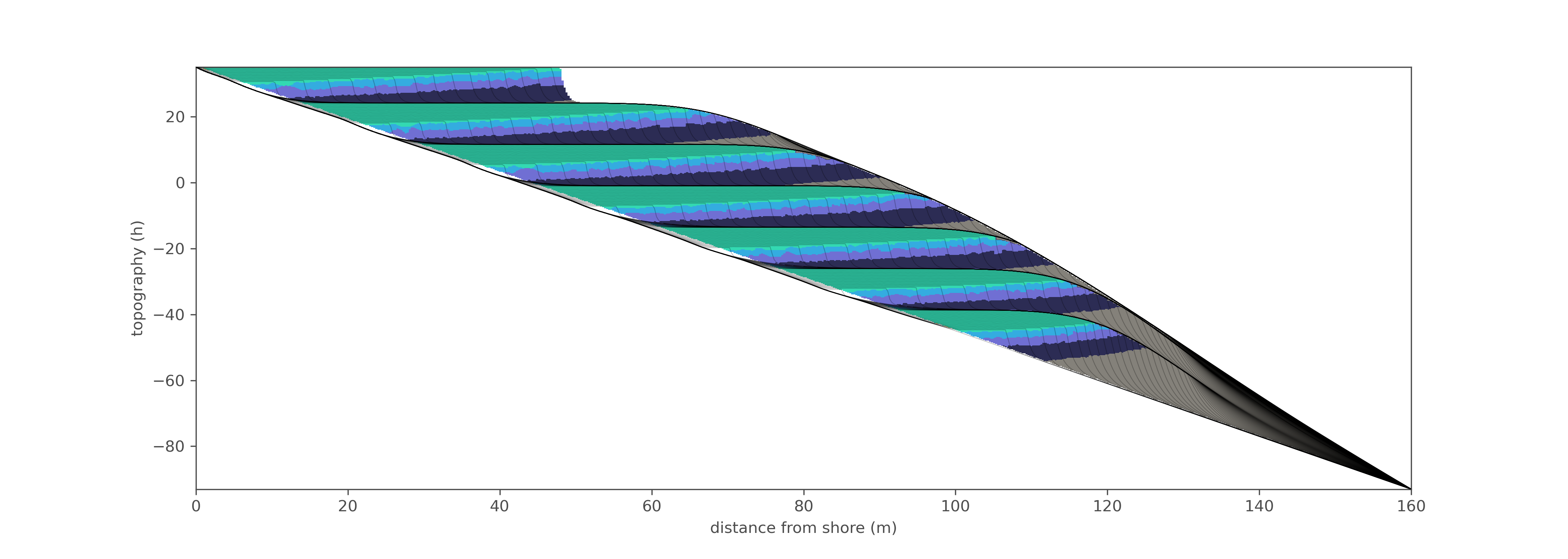
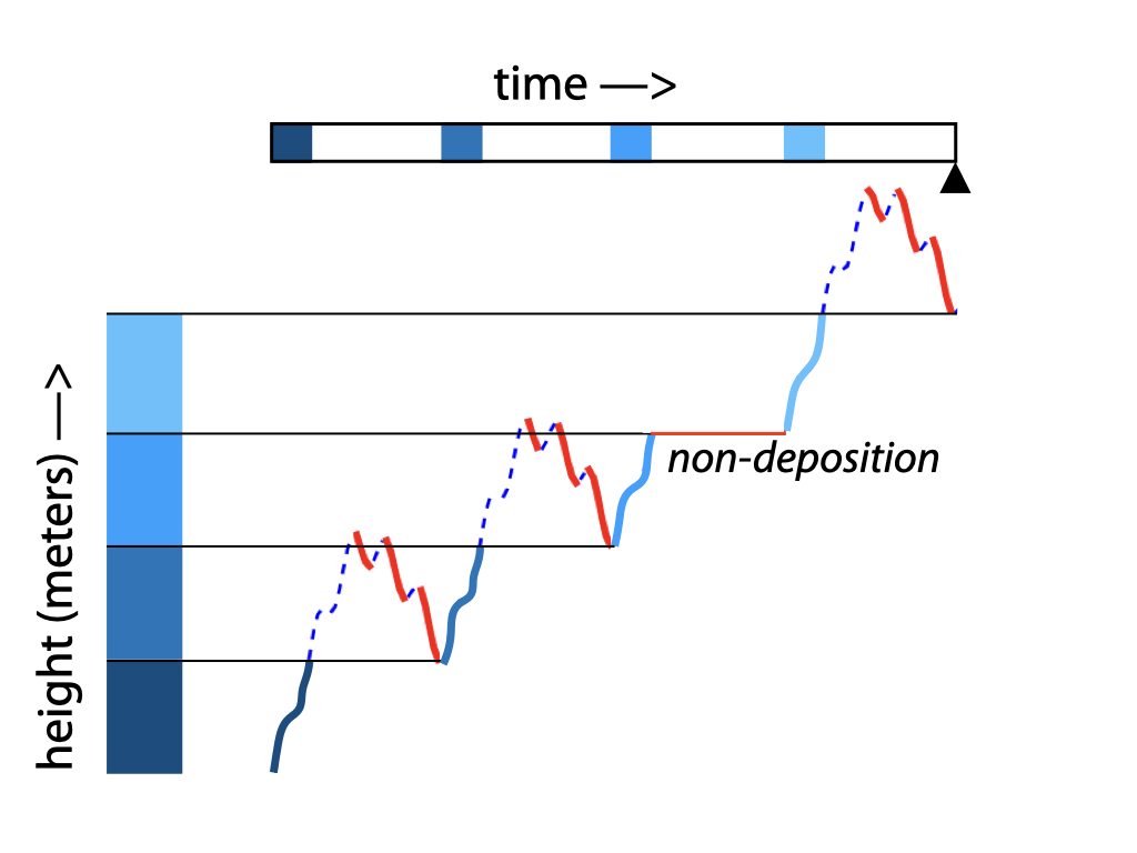
net sedimentary record is full of gaps: both erosive surfaces and hiatuses.

How much time is represented by sedimentary rock?

• unless we can recognize these surfaces, net sedimentation looks pretty continuous
• in fact, only 25% of the elapsed time is represented as ROCK
• remainder is contained in the gaps!

How to build the net rock record

import csv
import numpy as np
from matplotlib import pyplot as plt
import seaborn as sns
sns.set_context('talk')
%matplotlib inline

#empty lists for data
model_topo=[]

#open the data file
with open("model_results.csv","r") as fid:
    data = csv.reader(fid, delimiter=",")

    #reads the data in line-by-line
    for row in data:
        model_topo.append([float(r) for r in row[1:]])

#convert to list of numpy arrays
model_topo=[np.array(t) for t in model_topo]

#define as change from inital conditions 
model_topo=[t-model_topo[0] for t in model_topo]

• now lets see how we can build the net rock record from our diffusion model outputs - this is something that is needed for Assignment 1.3, question 2
• importing model topography (measured at 1000 grid points) through time (201 timesteps)
• first defining topography as DIFFERENCE in topography between end and beginning of model

How to build the net rock record

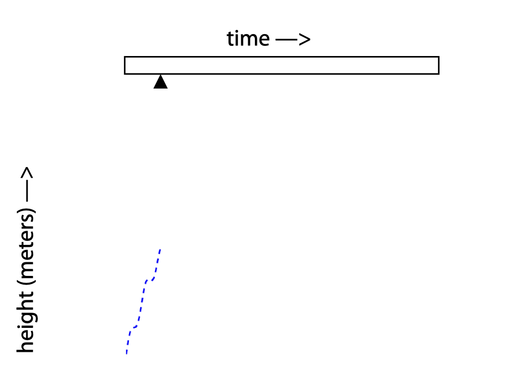
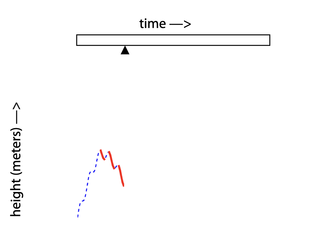
#pull topographic evolution from one spot in the basin
section=[t[454] for t in model_topo]

plt.plot(section,'-',color='r')
plt.plot(np.arange(len(section))[0::4],section[0::4],'.',markersize=5,color='k')

plt.gca().set_xticks([])
plt.gca().set_xlabel(r'time $\rightarrow$')
plt.gca().set_ylabel('height (meters)')
plt.gca().xaxis.set_label_position('top')  

• so let's plot up topographic evolution for one grid point (in this case, its 4.54 kilometers into our basin)
• can people spot the periods of erosion and/or hiatuses? Mark them up!
• so how do we go from this trajectory to the net rock record? has anyone made progress on this question?
• I will show one way, might not be the best way
• helpful to work BACKWARDS - start at the end, and burrow your way to the beginning
• at each black dot, look backwards in time - has topography INCREASED or DECREASED?

How to build the net rock record

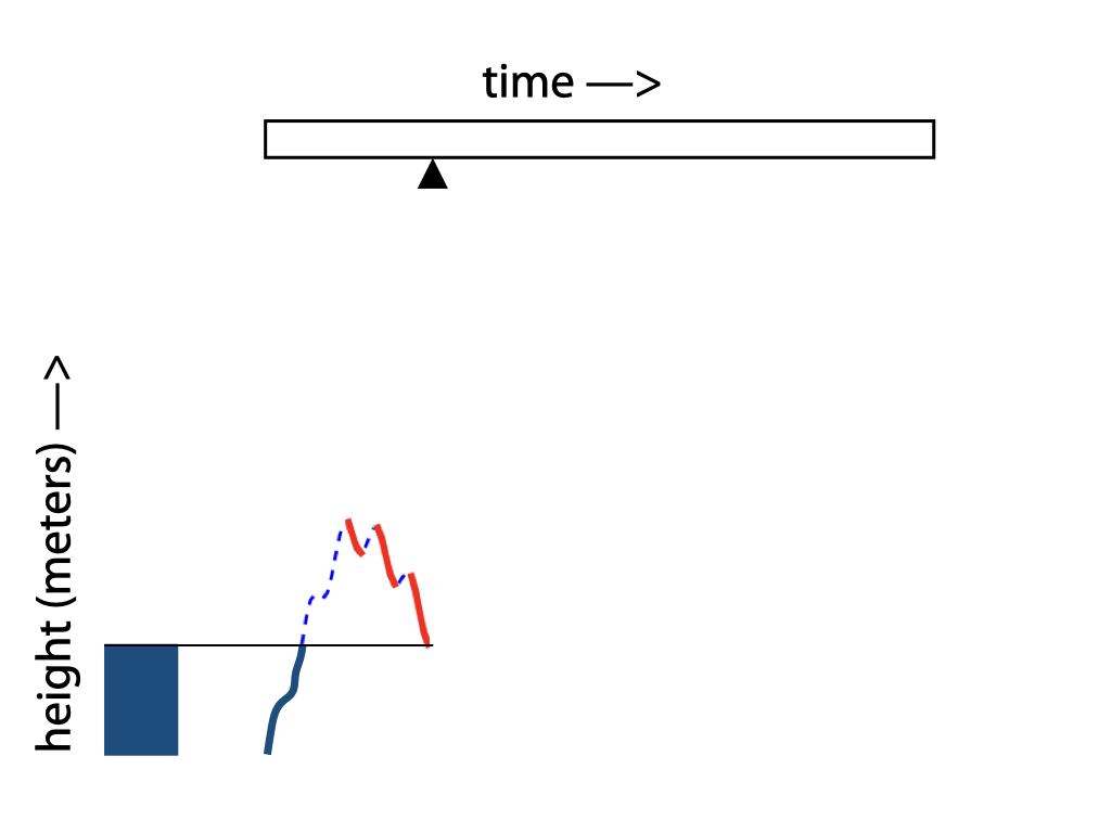
net=np.flipud(section) #flip this stratigraphy upside down to examine youngest to oldest
for i,s in enumerate(net): #count through time slices starting at the youngest
    if i!=len(net)-1: #if we're not at the end
        #look "down section" - was this layer eroded?
        # --> if height had decreased, then yes
        if s<net[i+1]: #s is height of current timeslice, net[i+1] is heigh of previous timeslice
            net[i+1]=s #create new record of net sedimentation
#make stratigraphy younging upwards again
net=np.flipud(net)
plt.plot(net,color='b')
plt.fill_between(np.arange(len(section)),section,net,color='r',alpha=0.25)
plt.gca().set_xticks([])
plt.gca().set_xlabel(r'time $\rightarrow$')
plt.gca().set_ylabel('height (meters)') 
plt.gca().xaxis.set_label_position('top') 

• this is exactly what this code is doing for this particular section location
• plot it up, and we can see that we've identified the period of erosion

How to build the net rock record

• so I have applied that same algorithm throughout my model basin, and this allows me to make strat sections like this
• can also mark EROSIVE SURFACES and NON-DEPOSITION SURFACES (which are sometimes called hardgrounds, especially when dealing with carbonate lithologies)
• each erosive surface is marked by how much sediment was created and then later destroyed
• this is the "field geologists" view of things.
• Imagine we had a slice through our model basin. Finding its base (datum = 0m), and measuring up. Making notes about sedimentary features and structures to make some inference about water depth (wider boxes = shallower) and erosion surfaces / hiatuses

Coastline position and erosion and hiatus

We will look at a set of model runs to better understand the relationship of the coastline position to erosion and hiatus (and time). First, let's review the controls on coastline position:

• Coastline progrades/regresses/moves seaward when: $\frac{sed}{dt}>\frac{space}{dt}$
• Coastline retrogrades/transgresses/moves landward when: $\frac{sed}{dt}<\frac{space}{dt}$
• Coastline aggrades/stays in the same location landward when: $\frac{sed}{dt}\approx\frac{space}{dt}$

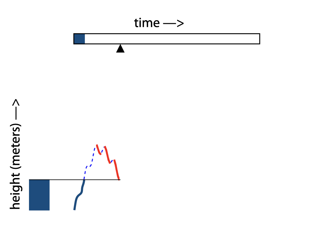
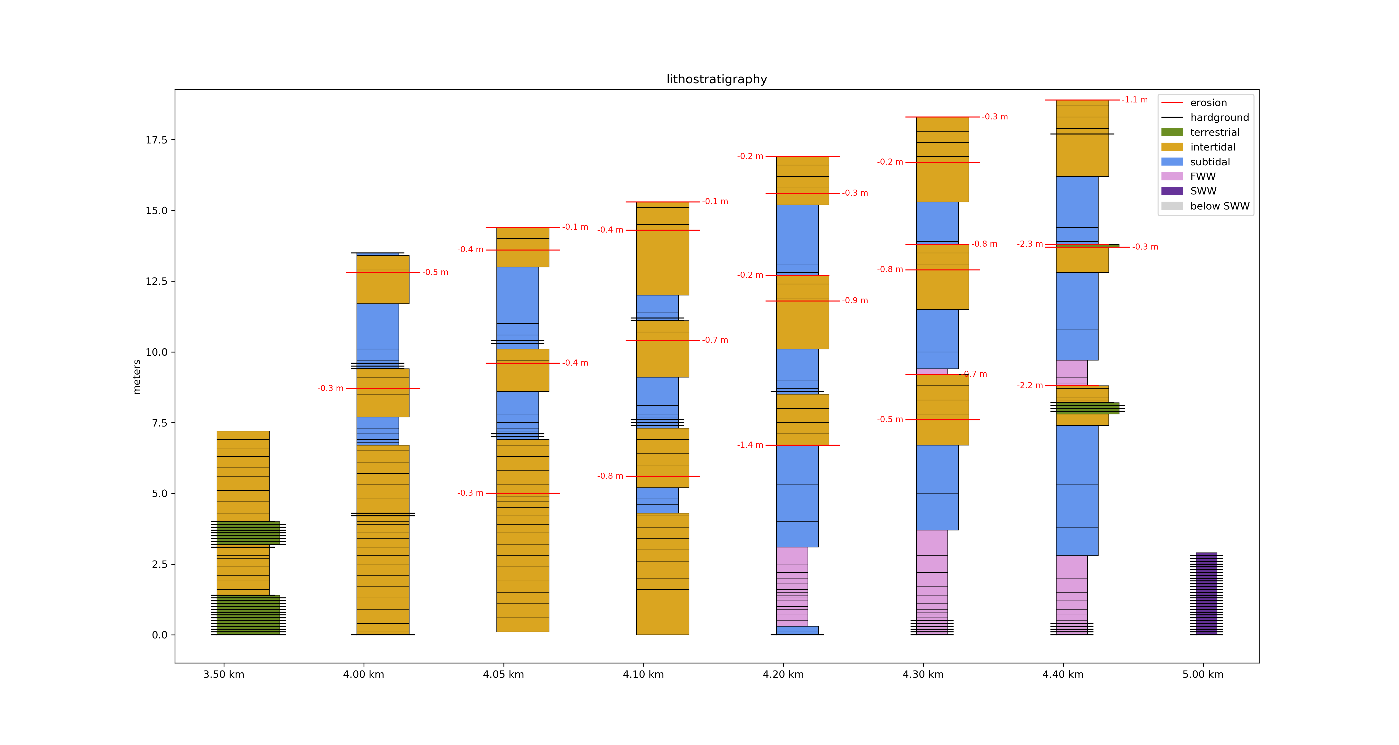
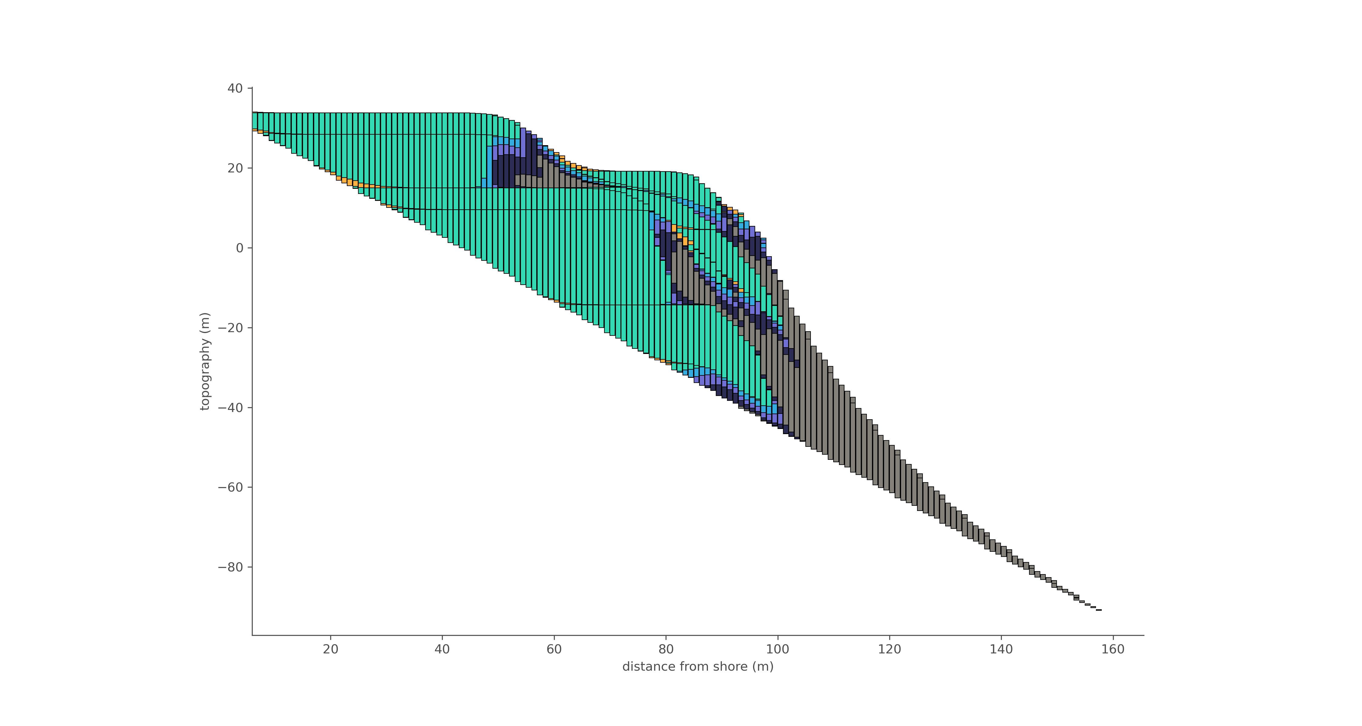
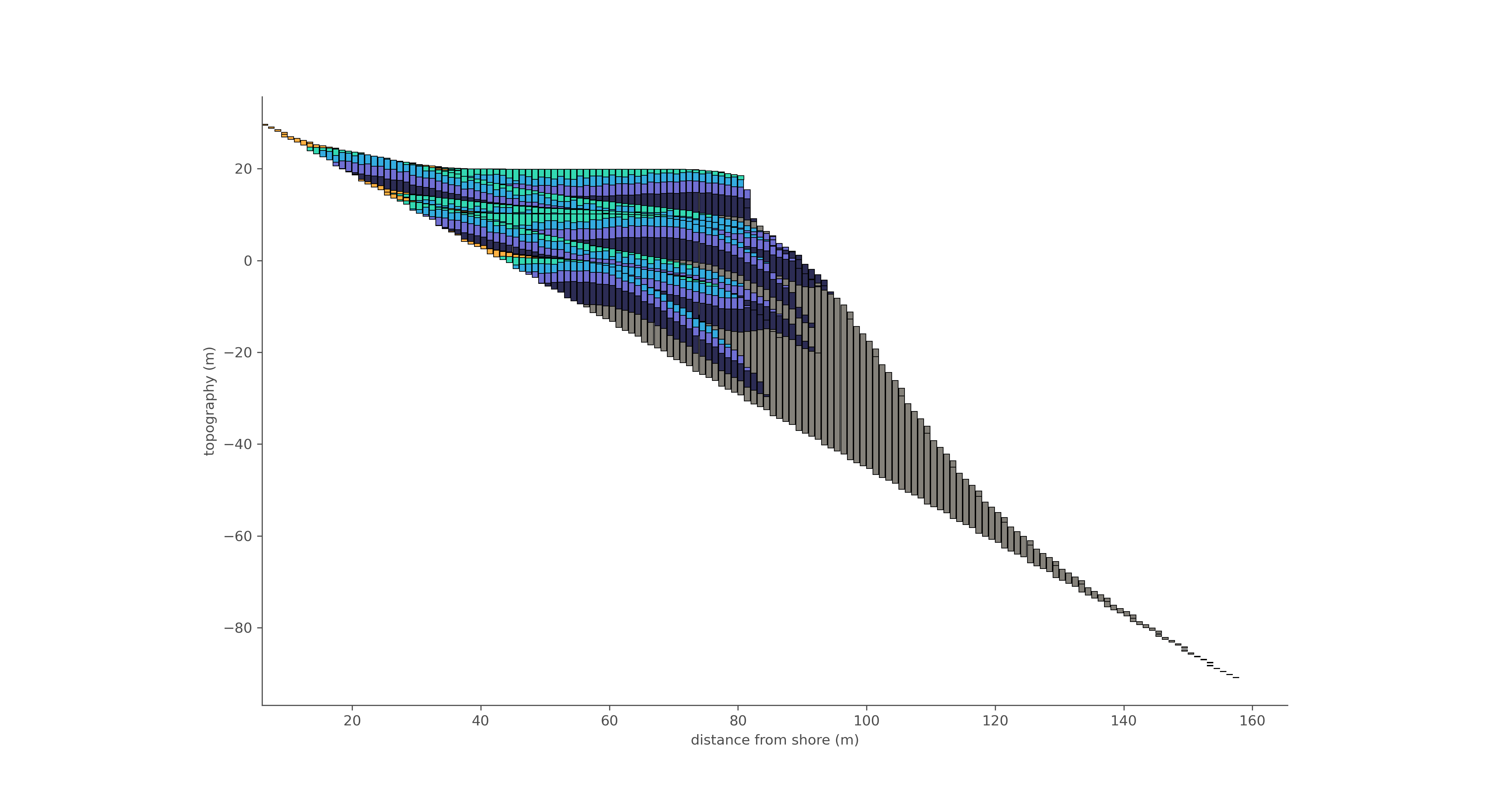
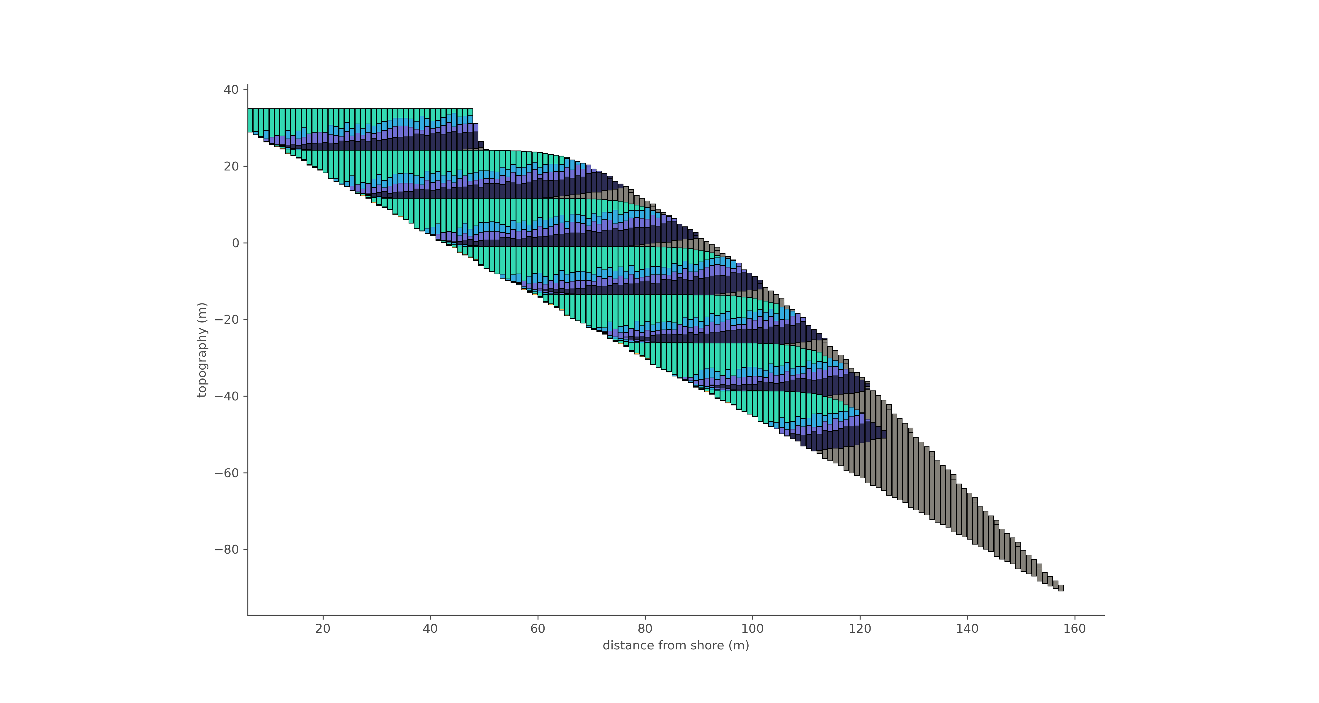
Simple sea level cycles: stratigraphic columns

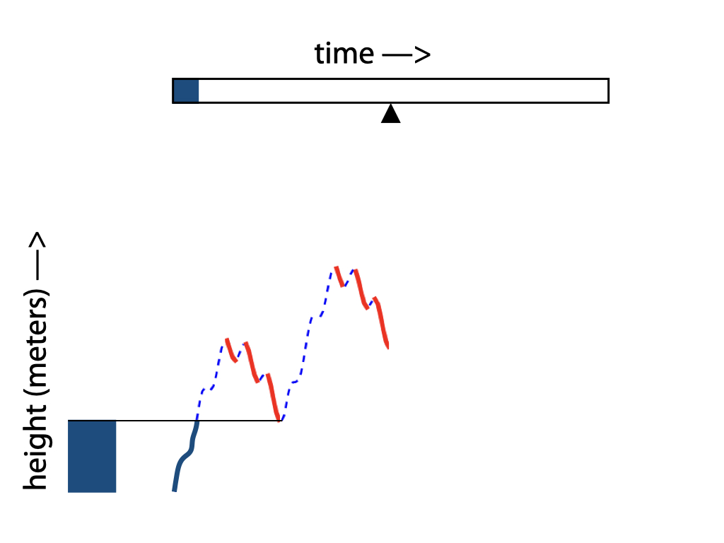
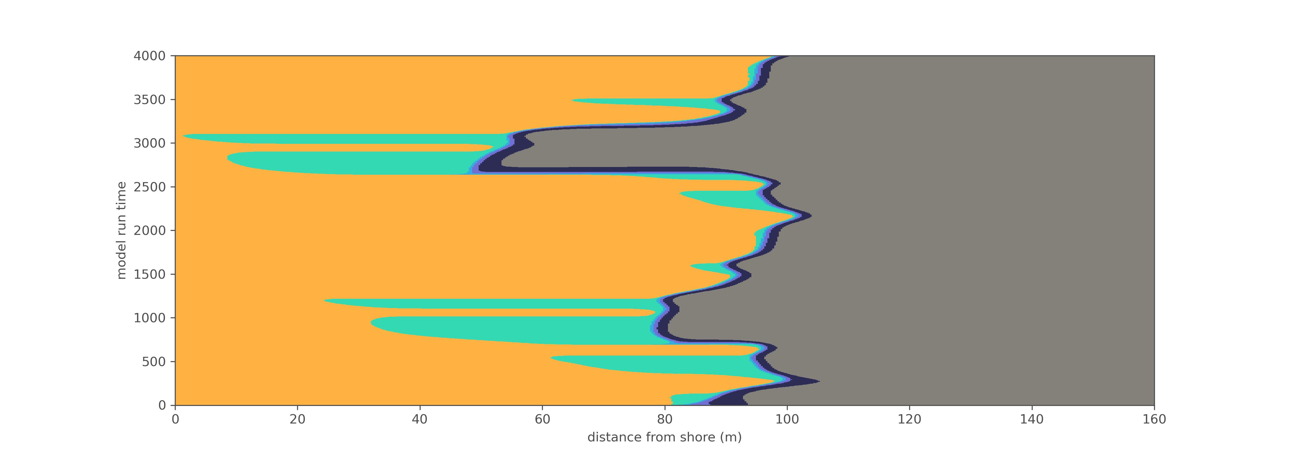
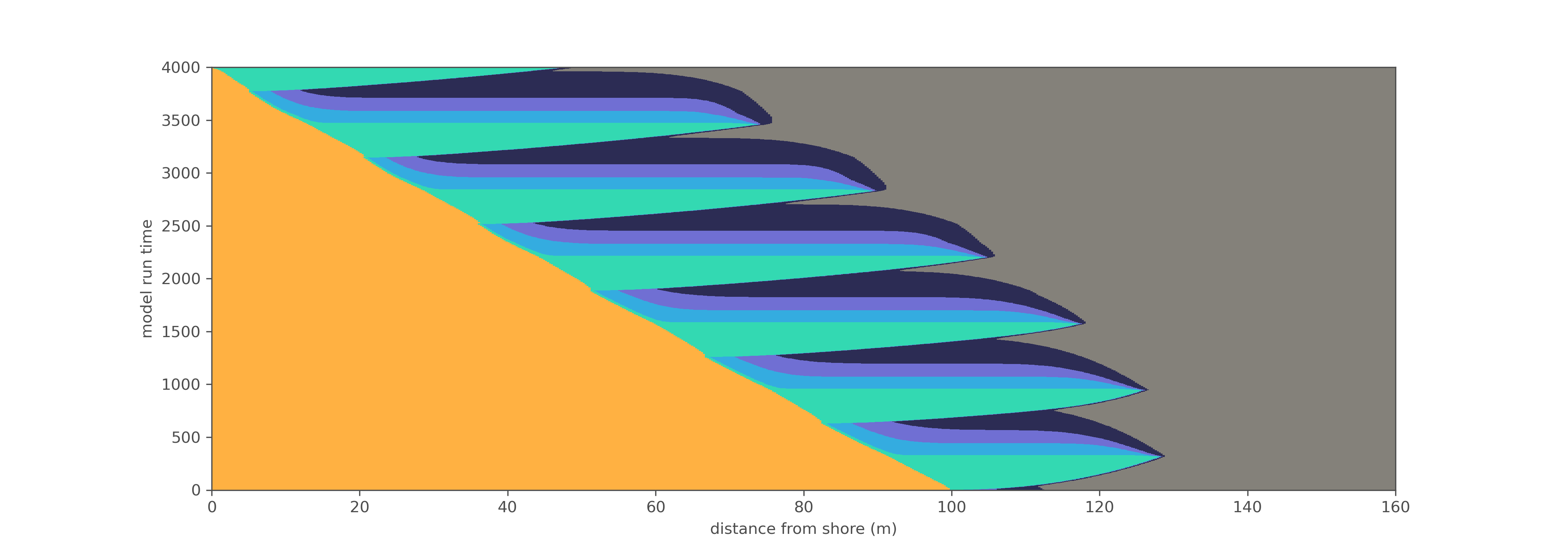
Simple sea level cycles: time vs topography

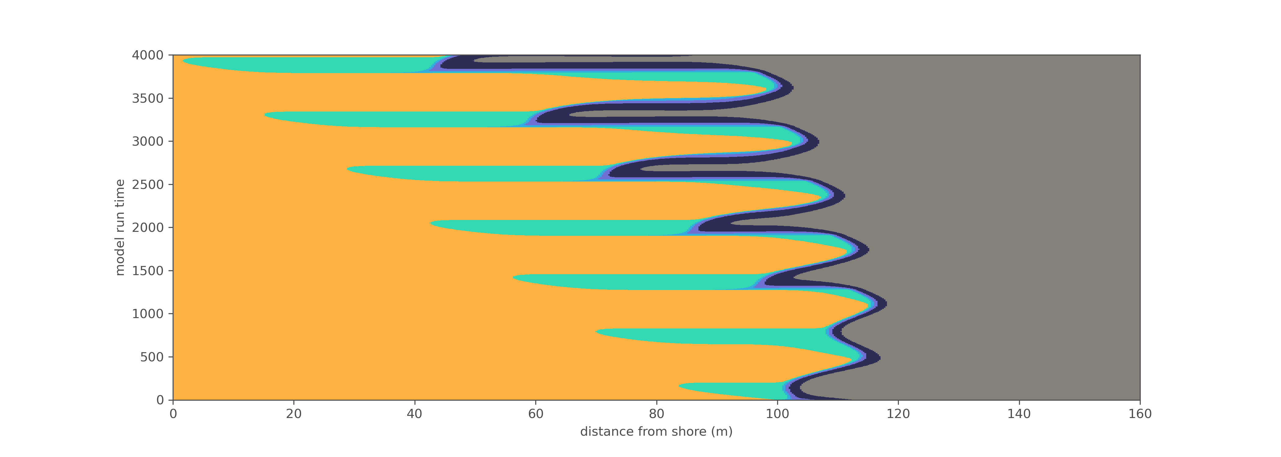
Simple sea level cycles: time vs topography

Where do you get erosion? Where is erosion rate maximized? What about non-deposition? (annotate/draw on your handout)

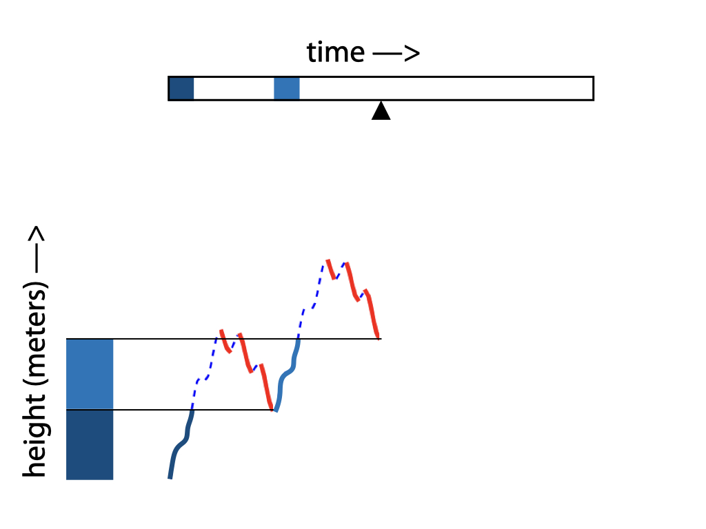
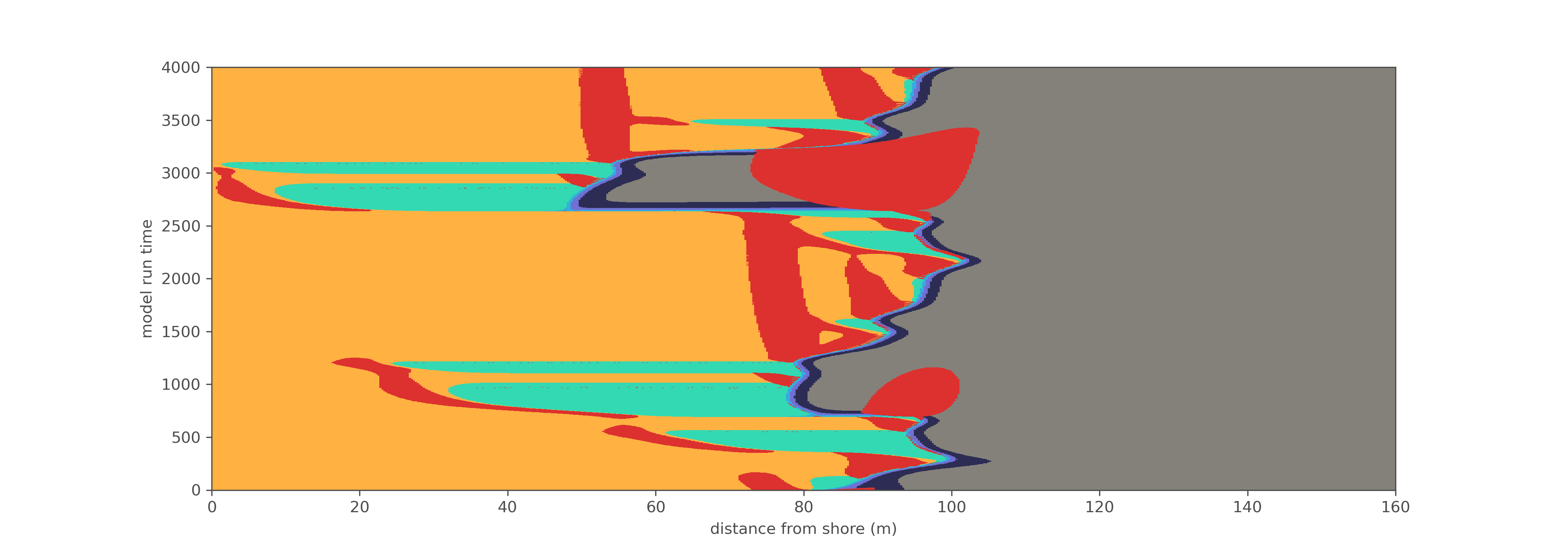
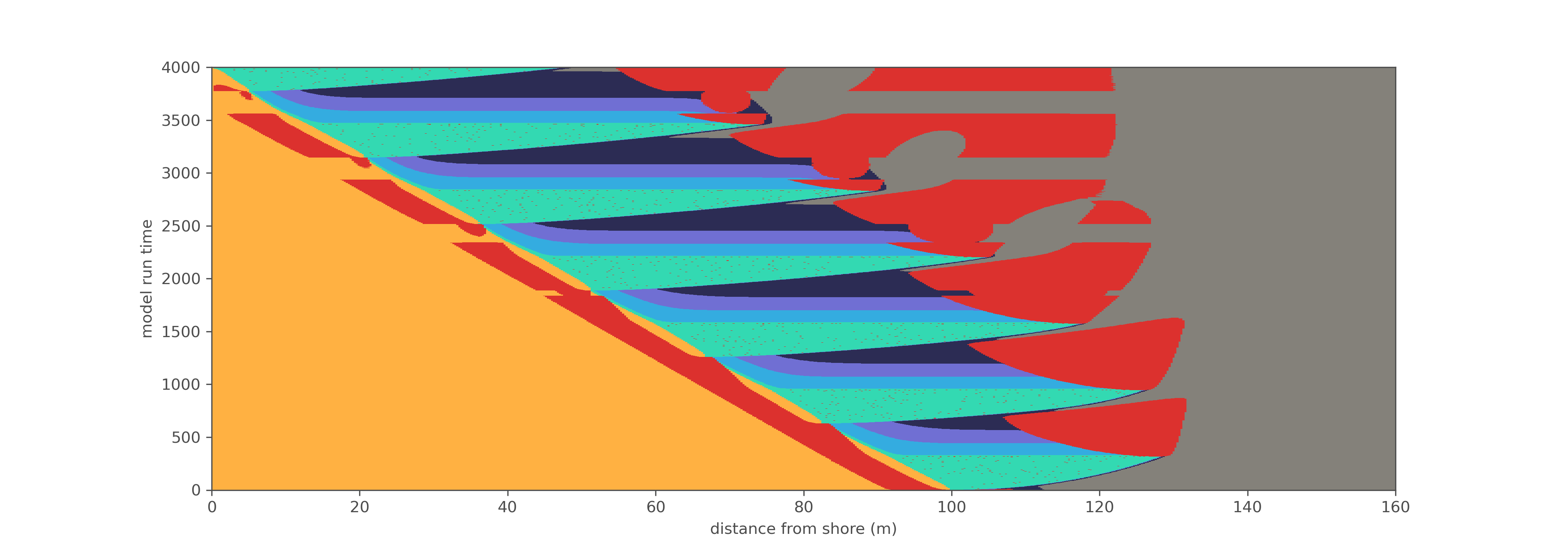
Simple sea level cycles: time vs topography (erosion)

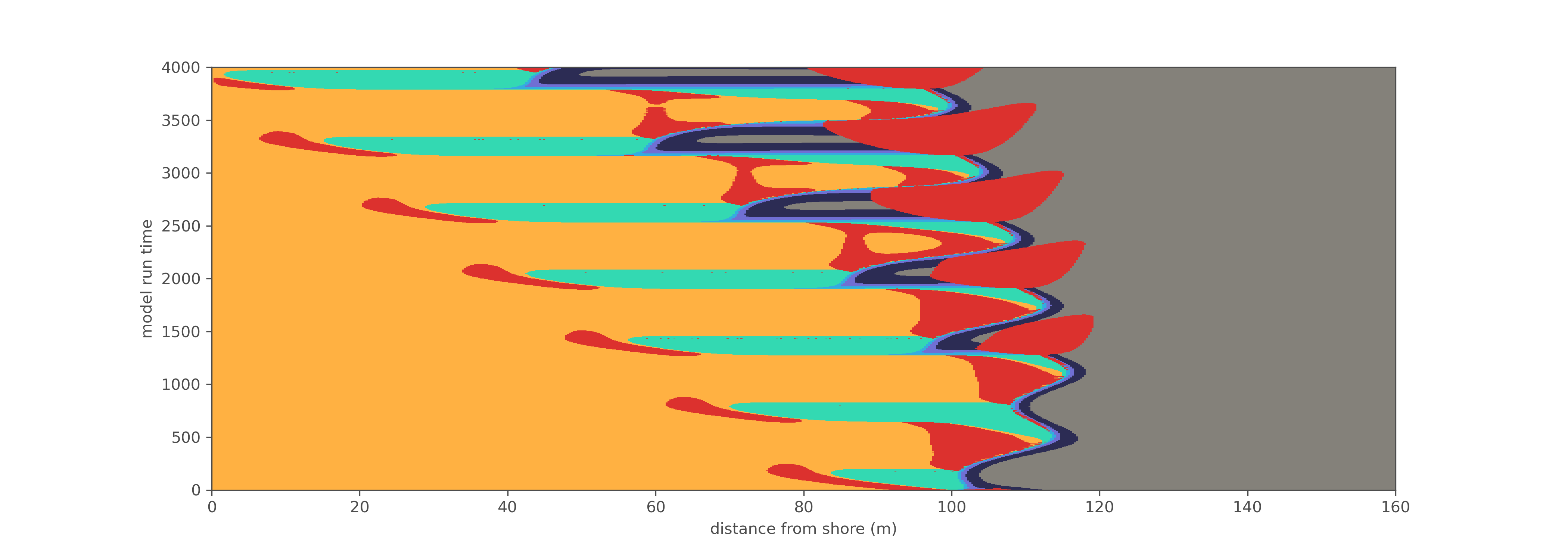
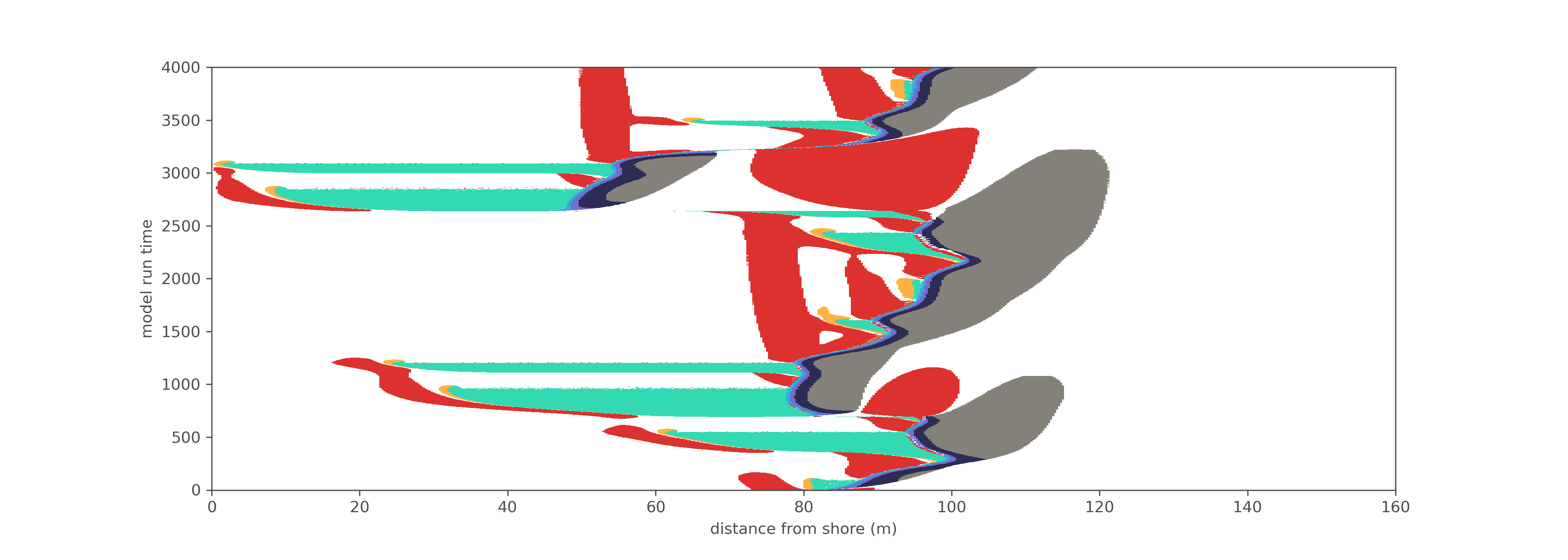
Simple sea level cycles: time vs topography (erosion and hiatus)

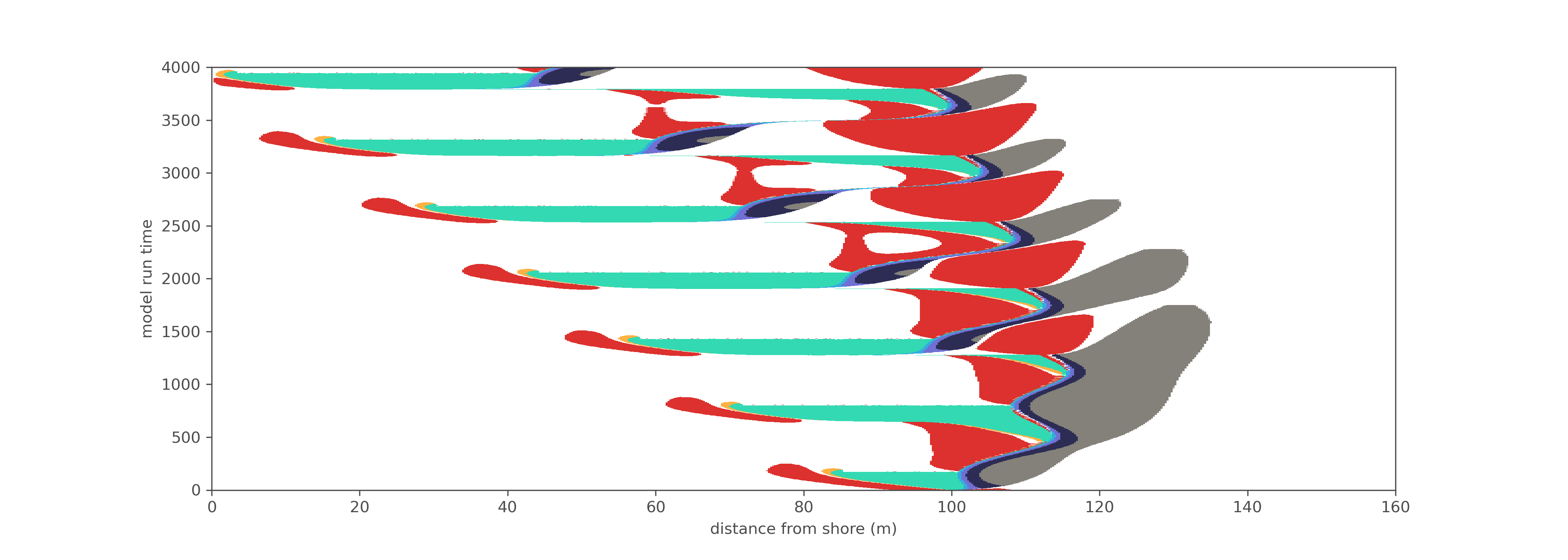
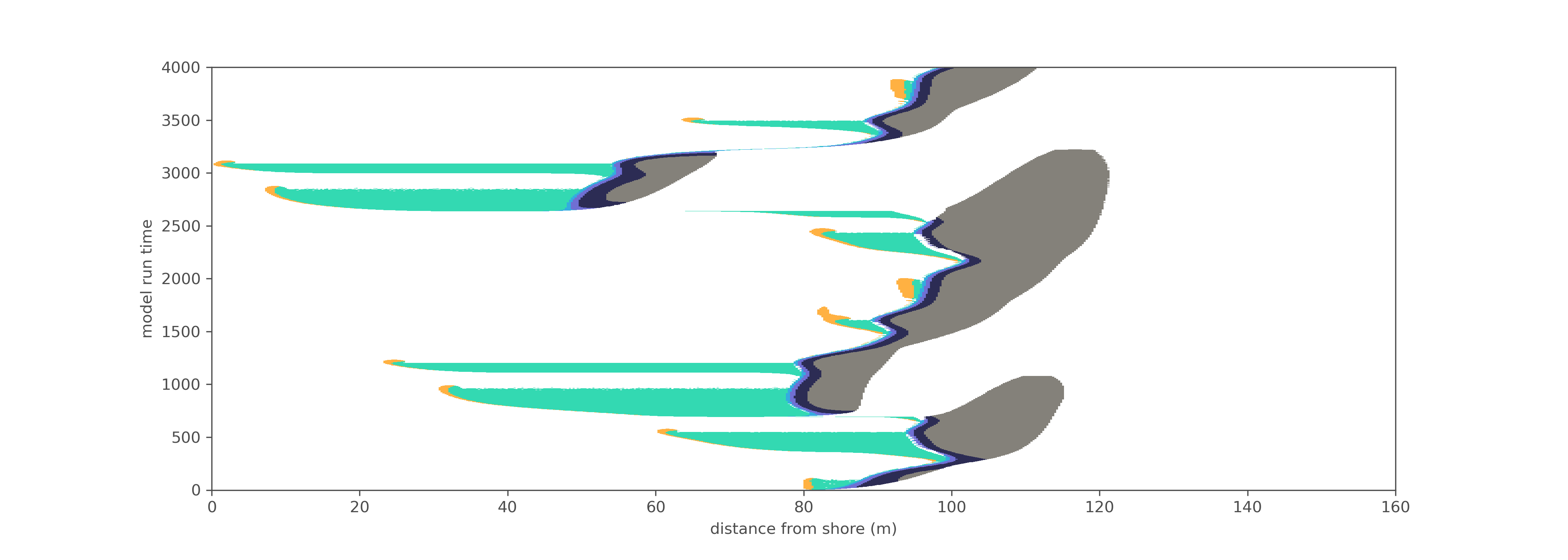
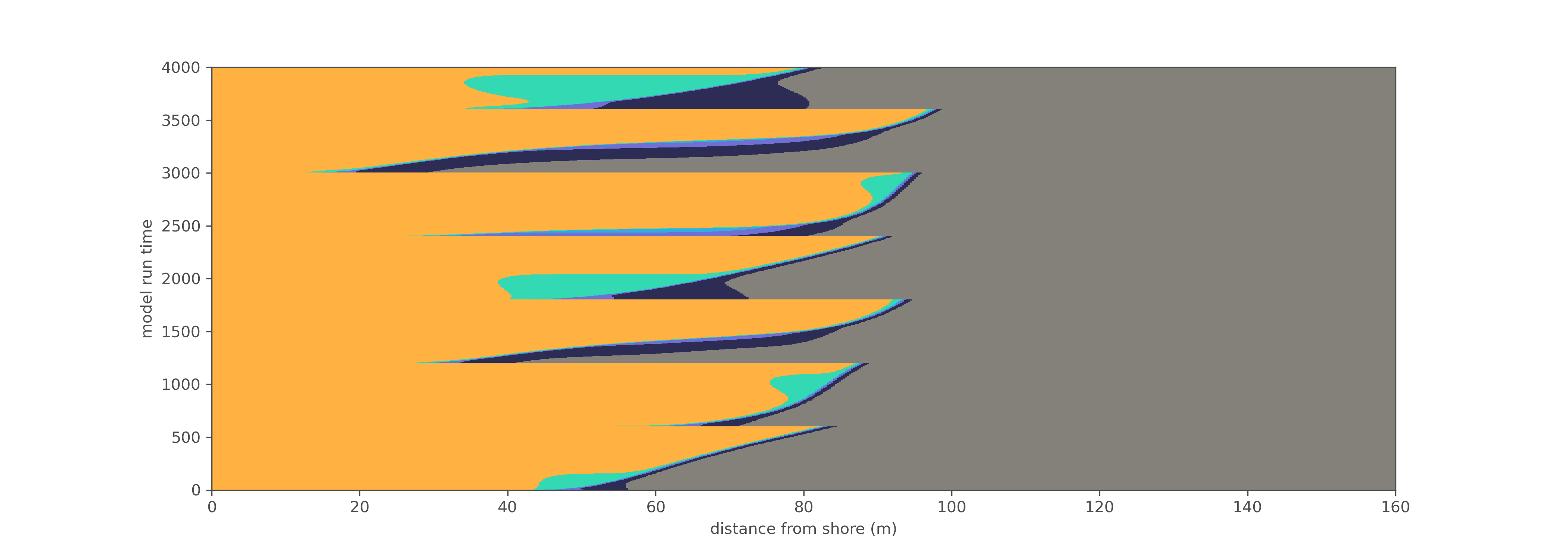
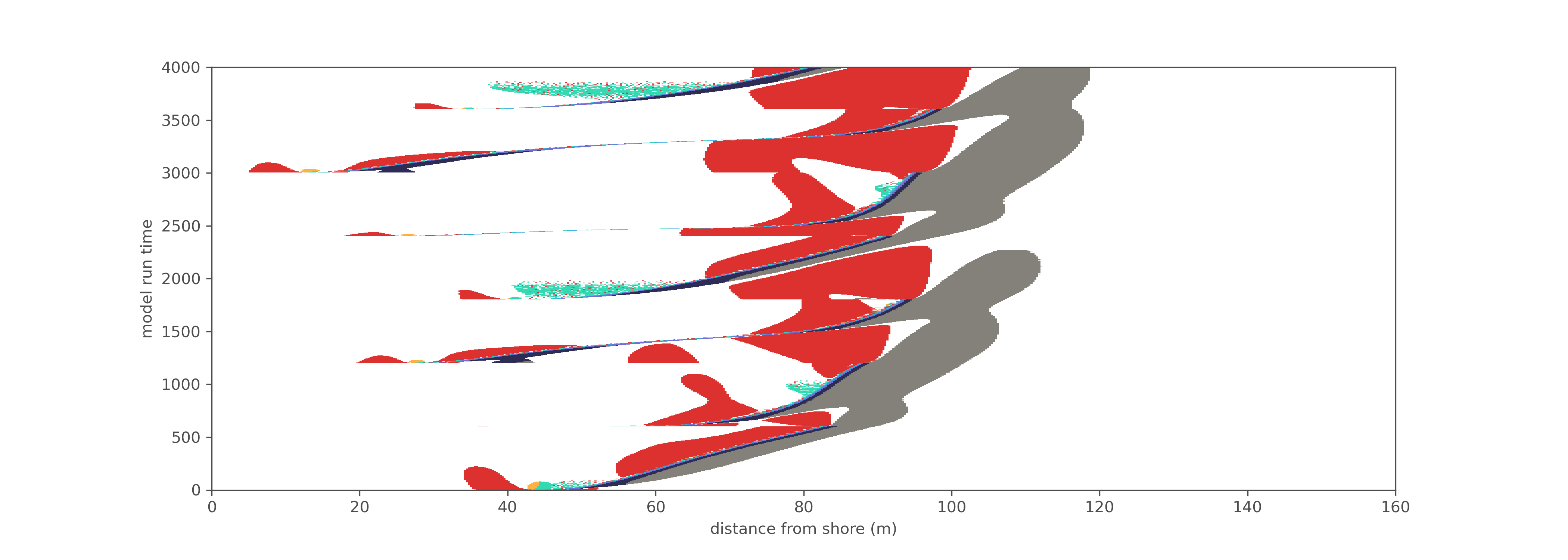
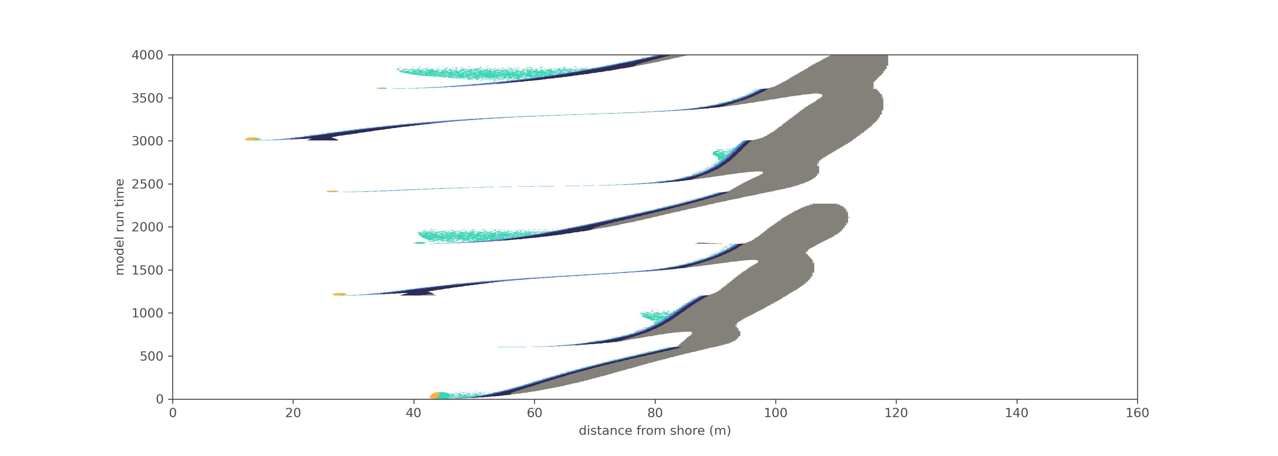
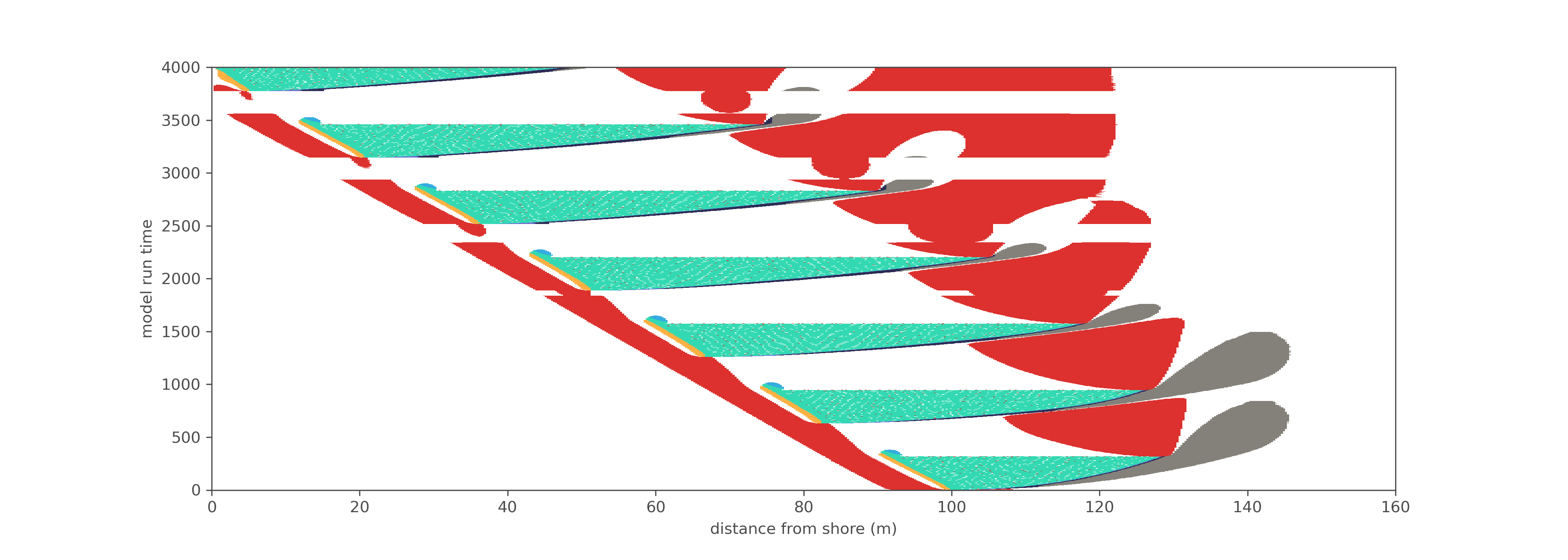
Simple sea level cycles: Wheeler diagram

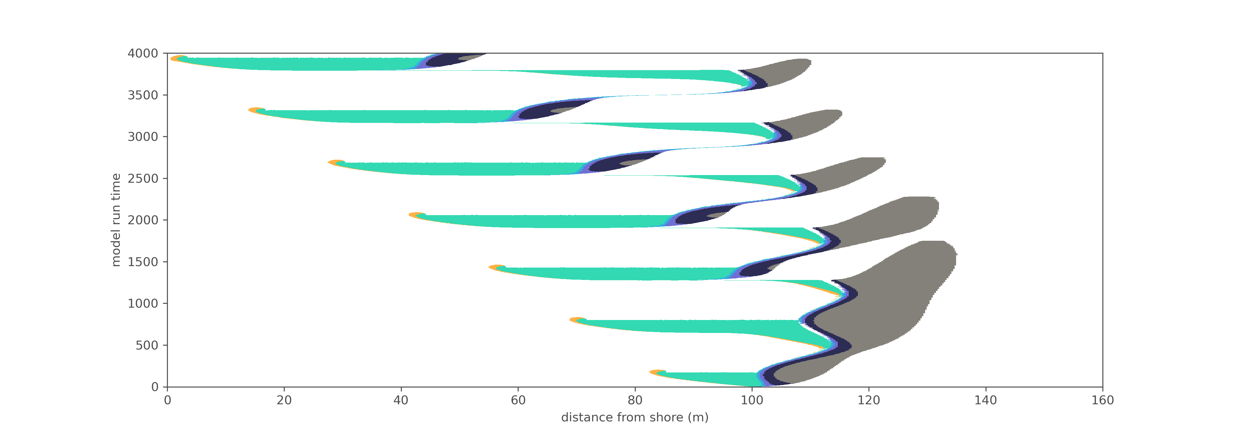
Simple sea level cycles: Wheeler diagram

Note: not all positive deposition is significant. Discuss where you think the thickest sediments (highest sedimentation rates) are.

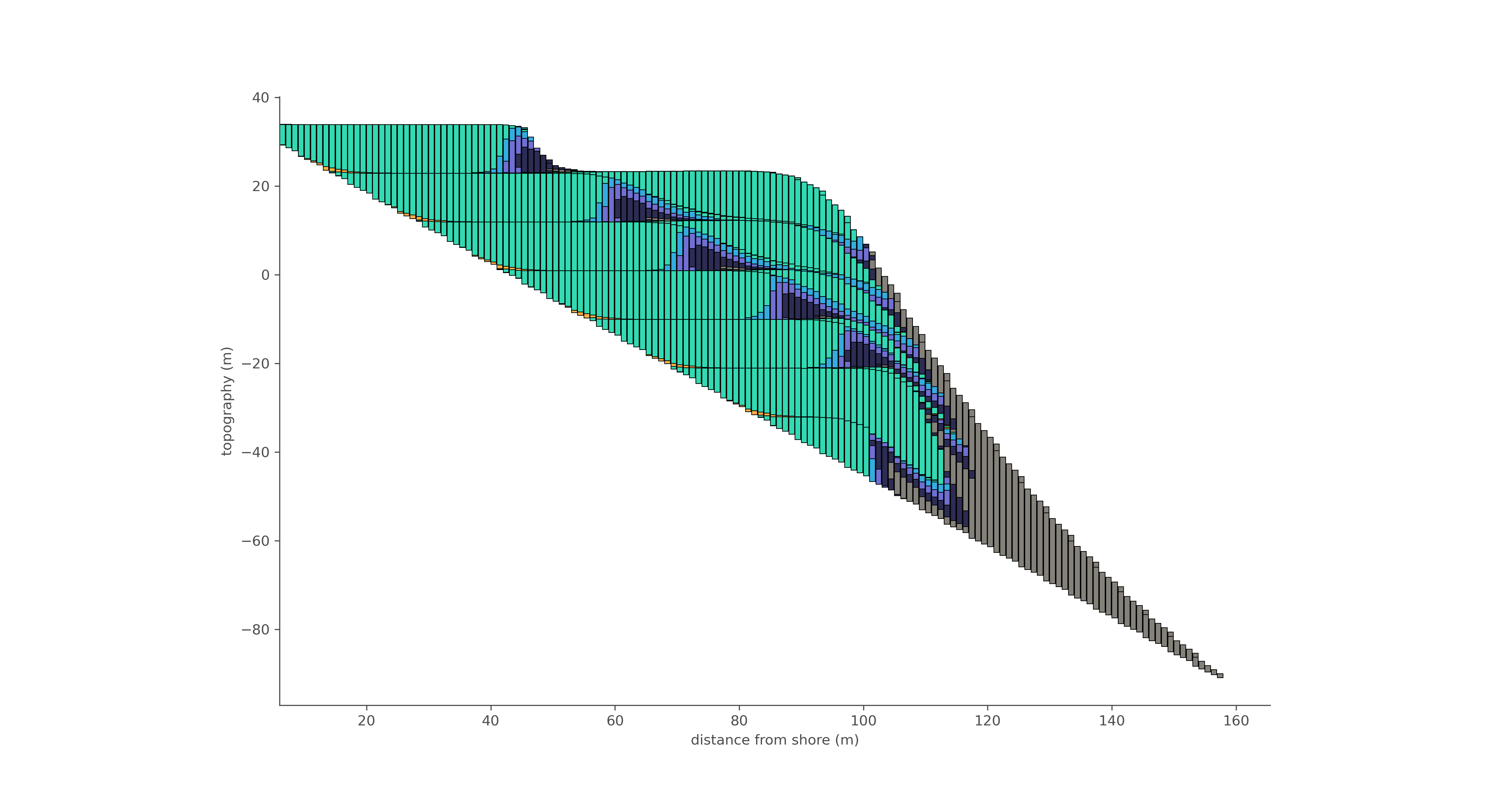
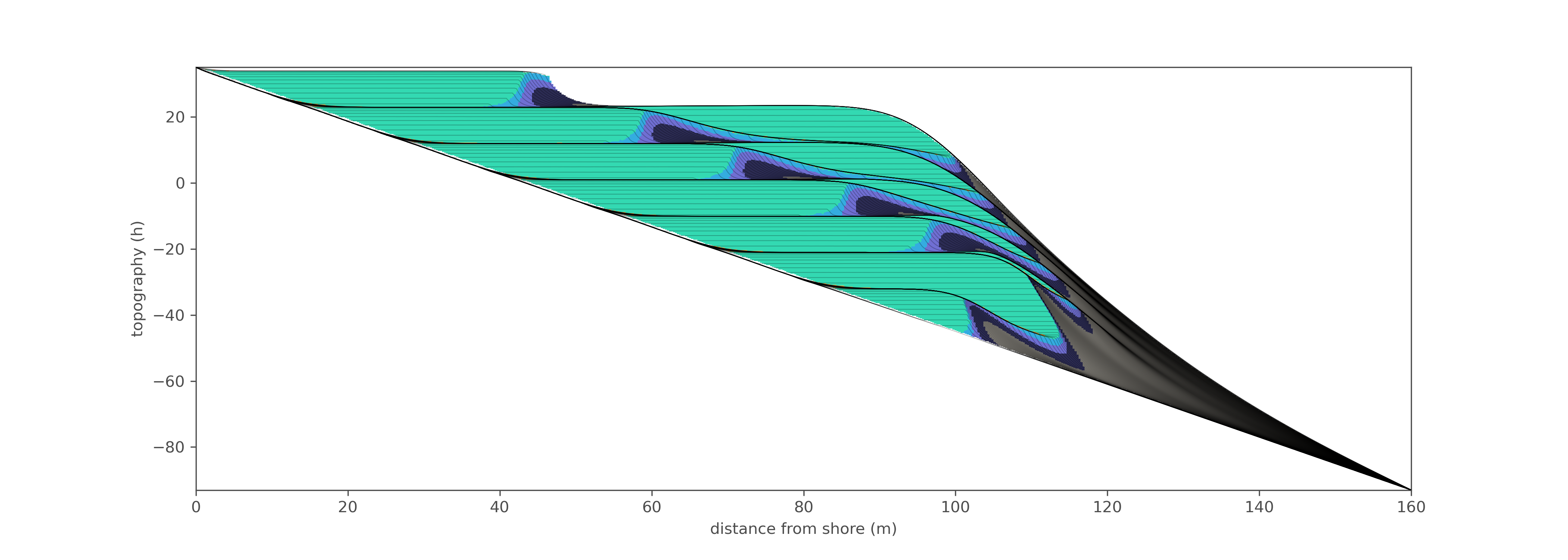
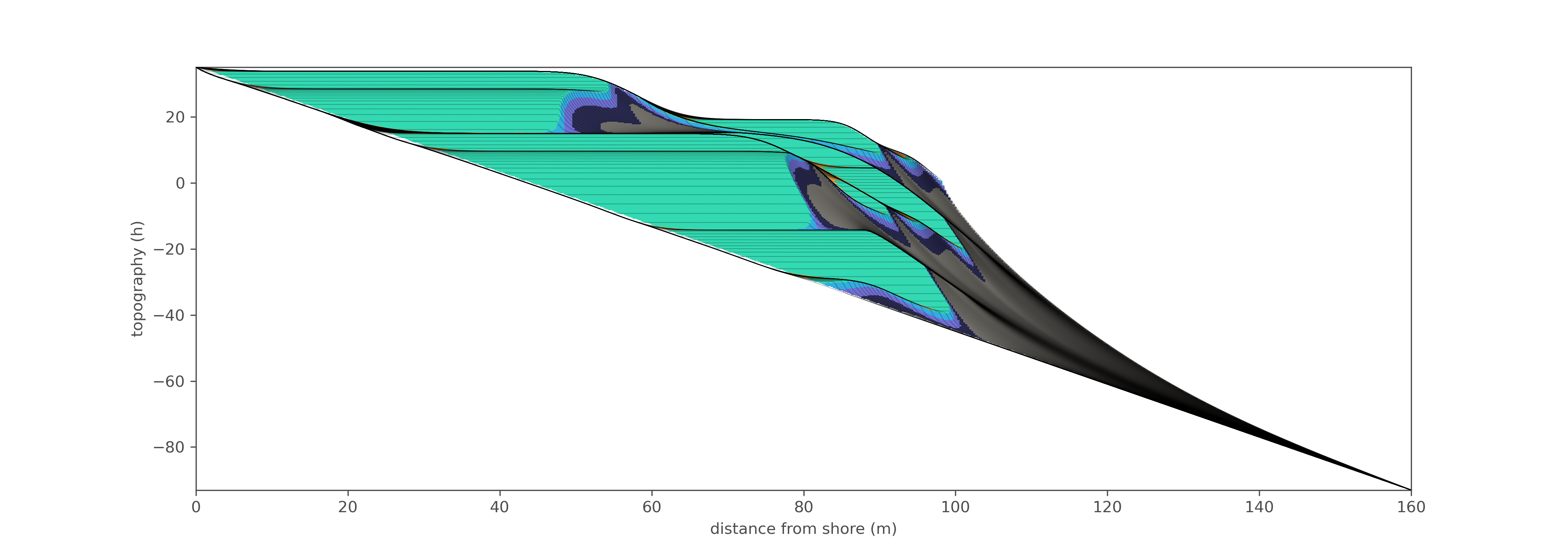
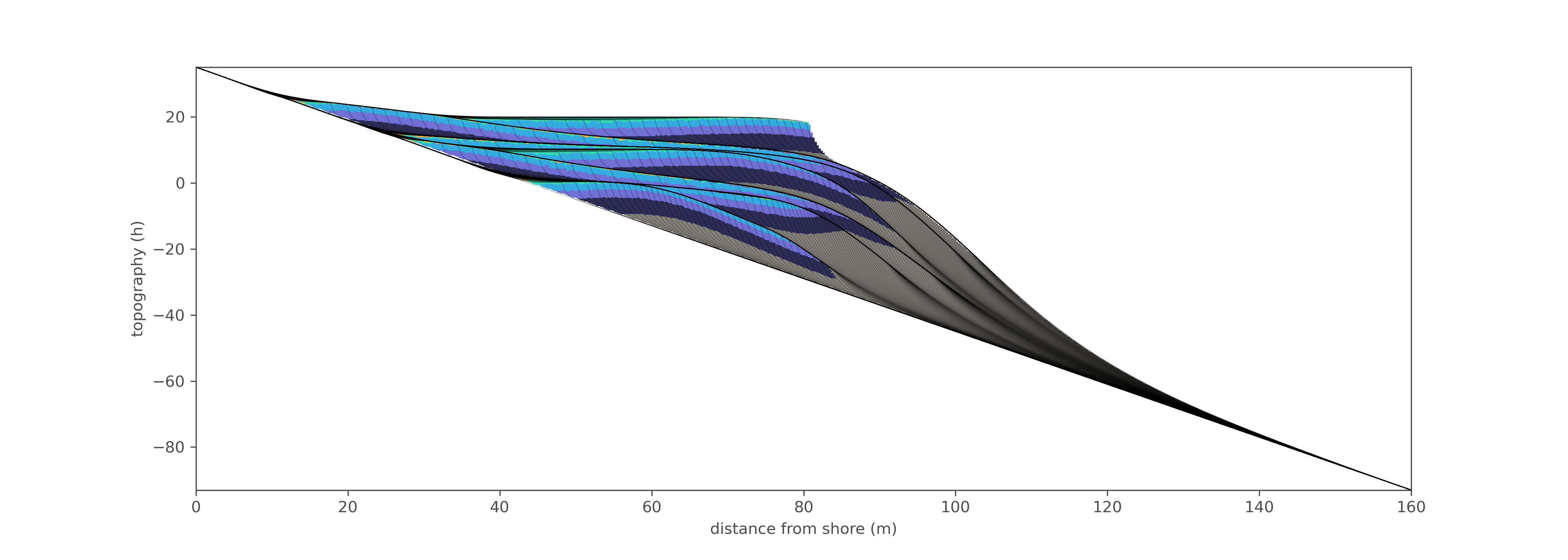
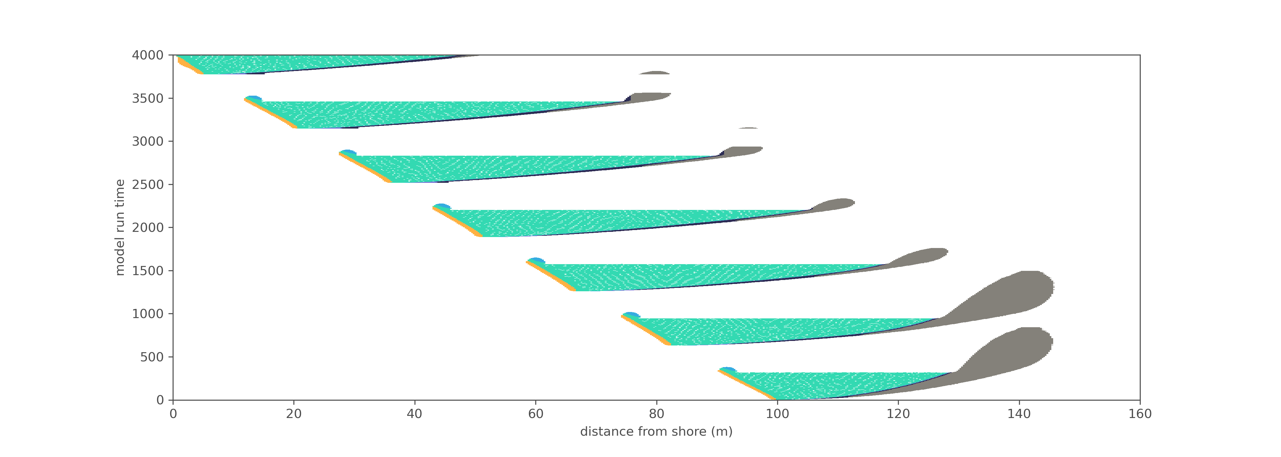
Simple sea level cycles: stratigraphic profile

Class example 1: stratigraphic columns

Class example 1: time vs topography

Class example 1: time vs topography (erosion)

Class example 1: time vs topography (erosion and hiatus)

Class example 1: Wheeler diagram

Class example 1: stratigraphic profile

Class example 2: stratigraphic columns

Class example 2: time vs topography

Class example 2: time vs topography (erosion)

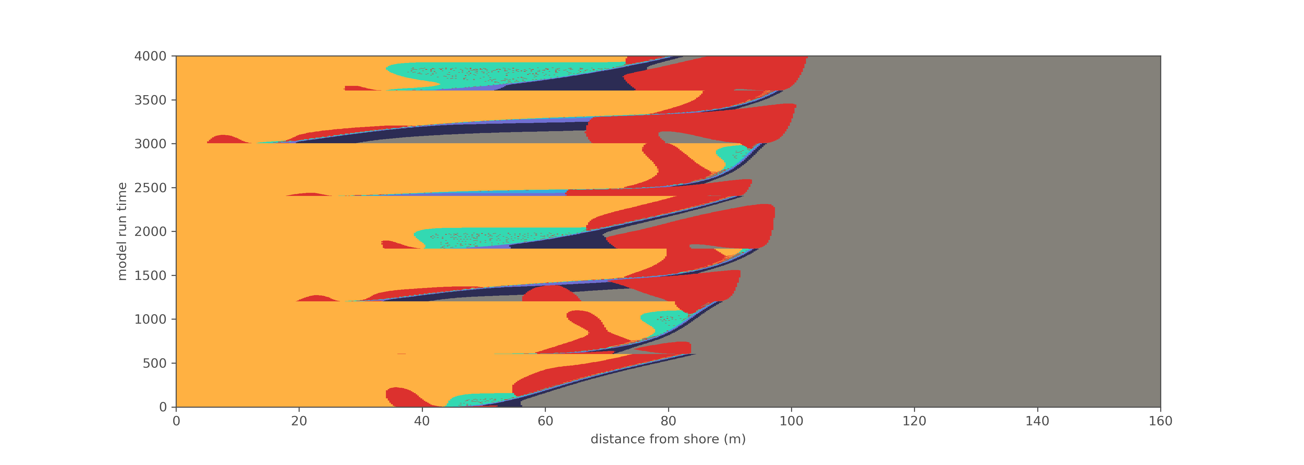
Class example 2: time vs topography (erosion and hiatus)

Class example 2: Wheeler diagram

Class example 2: stratigraphic profile

On/Off sediment supply with constant subsidence: time vs topography

On/Off sediment supply with constant subsidence: time vs topography

On/Off sediment supply with constant subsidence: time vs topography (erosion)

On/Off sediment supply with constant subsidence: time vs topography (erosion and hiatus)

On/Off sediment supply with constant subsidence: Wheeler diagram

On/Off sediment supply with constant subsidence: stratigraphic profile