Lecture 12: Introduction to Age Models

1. The importance of knowing time
2. Building an age model
   • Markov chain Monte Carlo approaches
   • constant sedimentation rates
   • varying sedimentation rates

We acknowledge and respect the lək̓ʷəŋən peoples on whose traditional territory the university stands and the Songhees, Esquimalt and W̱SÁNEĆ peoples whose historical relationships with the land continue to this day.

Importance of knowing time

• we have talked before about the difficulty of recovering signals from stratigraphic sections
• in the transport module, the challenge was primarily to correlate surfaces across the basin

Importance of knowing time

• transgressive regressive cycles are way clearer on a wheeler diagram
• can see the migration of the shoreline
  • basinward during progradation / sea level fall
  • landward during transgression
  • shoreline can be followed by just tracking intertidal deposits
• in addition to being able to qualitatively view the record more clearly, a time model also makes this data more amenable to quantitative analysis

Age models are important: how do we get them?

1. Cyclostratigraphy
2. Biostratigraphy
3. Absolute ages
   • U-Pb (volcanics), Ar-Ar (volcanics), Re-Os (sediments)
4. Signal matching
   • magnetostratigraphy
   • chemostratigraphy
5. Relative ages
   • Amino Acid Racemization

Biostratigraphy

• based on the unique, sequential, nonrepeating appearance of fossils through time

Biostratigraphy

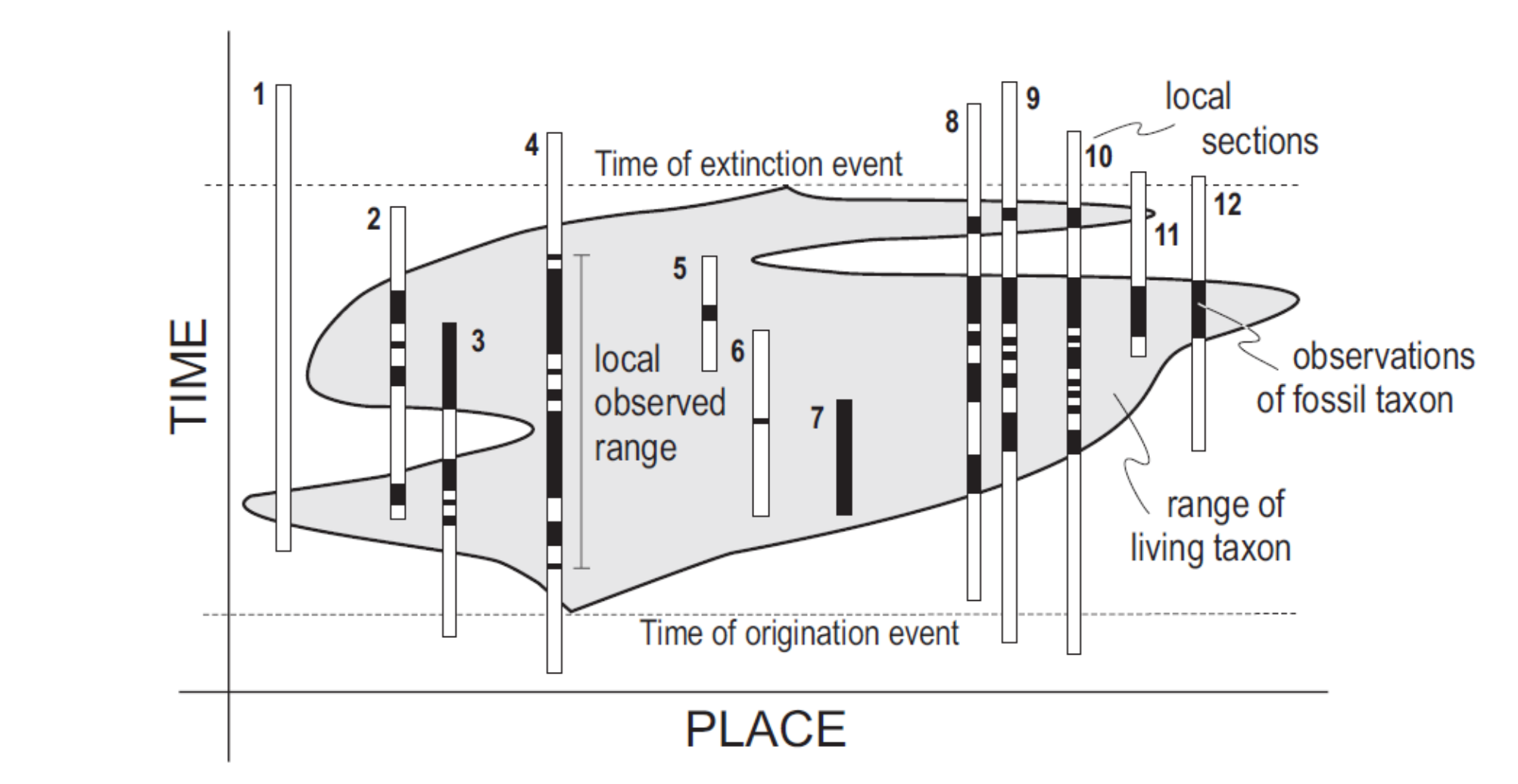
• based on the unique, sequential, nonrepeating appearance of fossils through time
• observations are: first appearance and last appearance per section

• most important are first appearance datums and last appearance datums
• in principle, a very simple concept

• what is wrong with this picture?
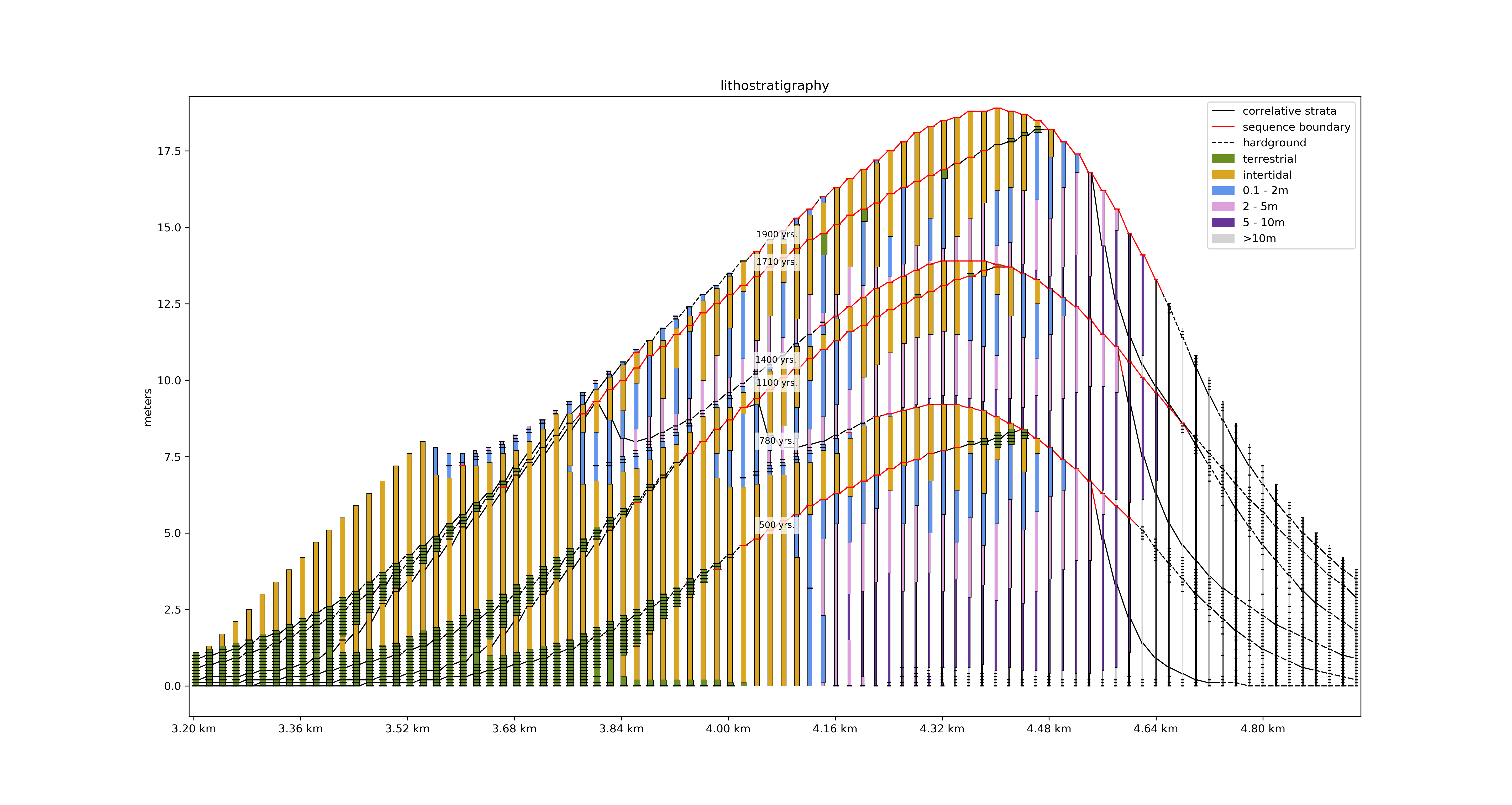
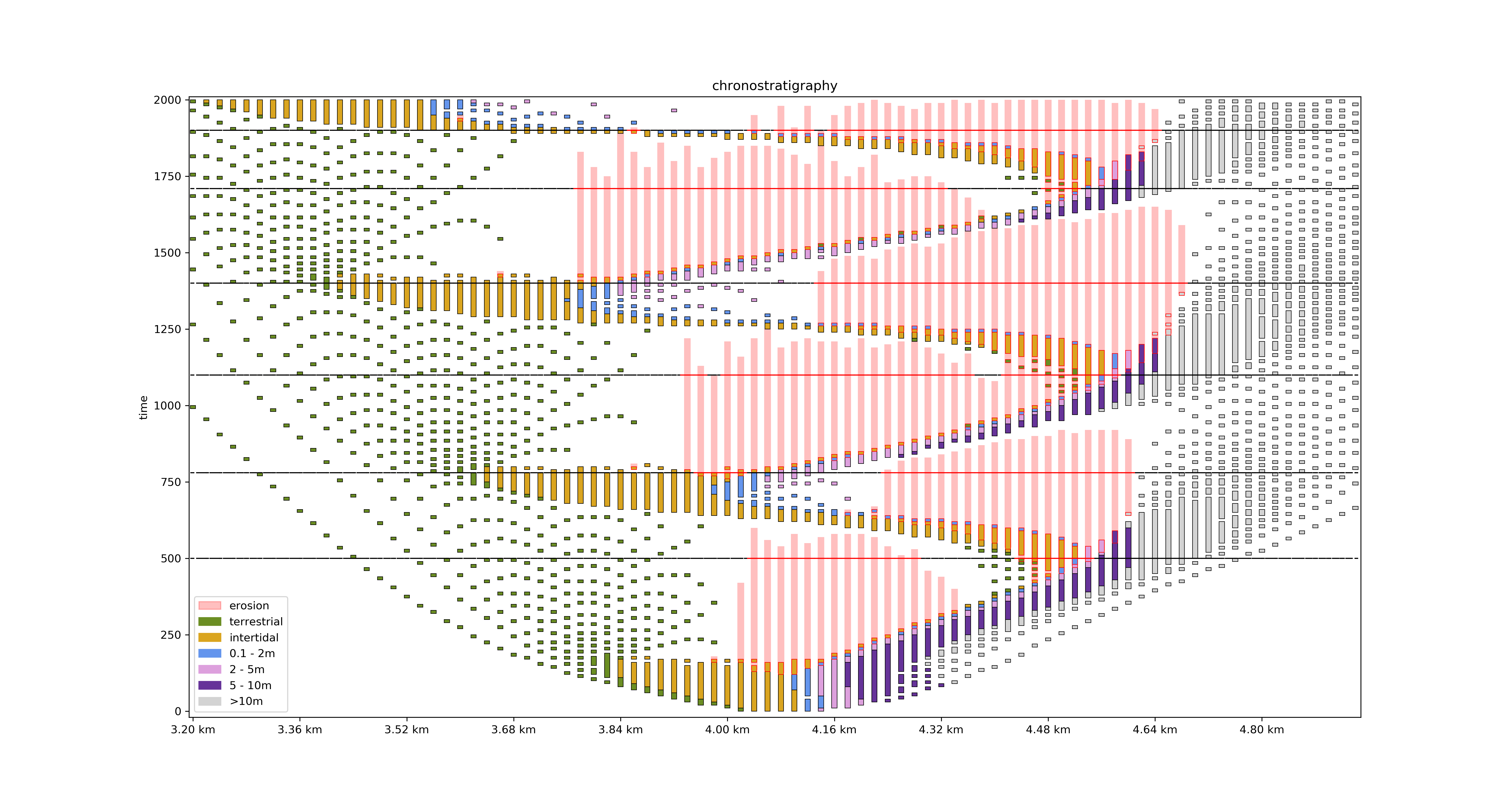
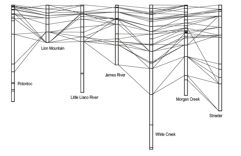
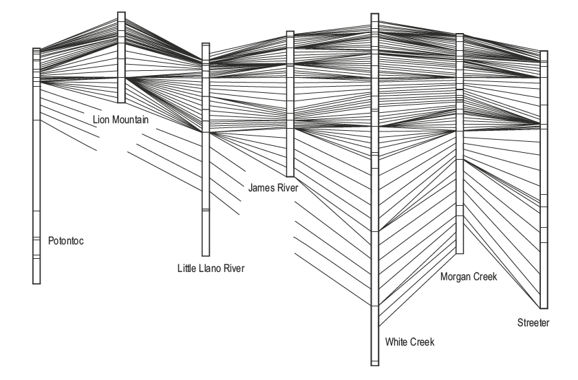
• fence diagram (correlation) of the observed FADs and LAD between 7 sections that preserve 62 taxa of the Cambrian Riley Formation of Texas (data from Palmer, 1954; Shaw, 1964).
• lines are meant to represent time lines, so equal time

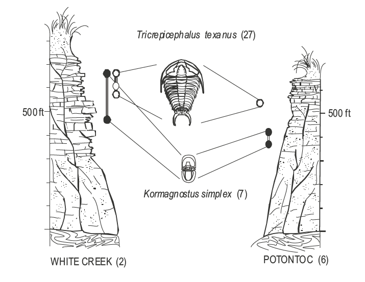
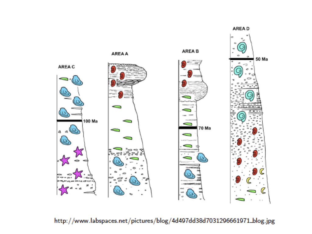
Contradictory ranges

• what could be causing this?

Contradictory ranges

• problems arise because relationship between taxa are not same in each section
• in this example, in one these taxa coexist, and in another, they do not
• ranges need to be MODIFIED to be consistent
  • assuming coexistence is real, then at section 6, this range needs to be extended

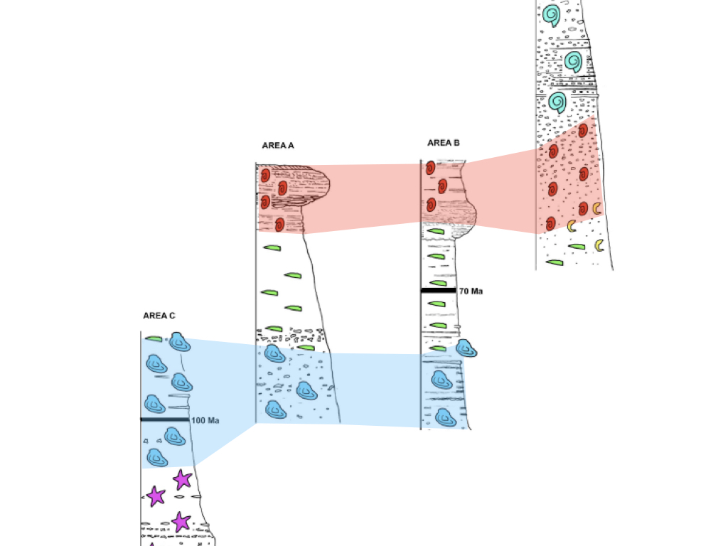
Resolving contradictory ranges

• ranges of original data need modifcation to be consistent everywhere (time goes left to right)

Resolving contradictory ranges

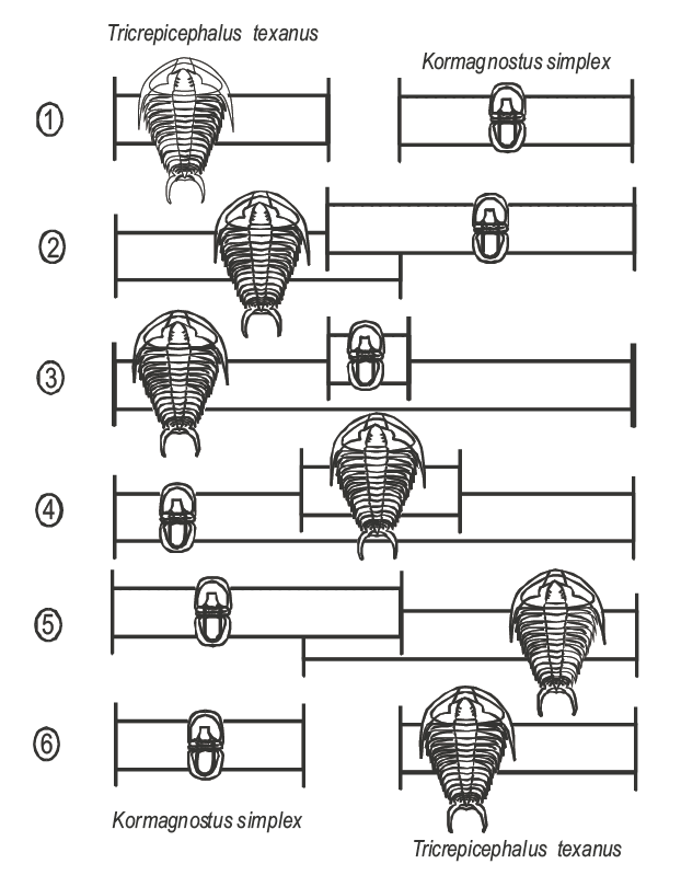
• can we rule any out? working out the possibilities not so hard with just two taxa..

Resolving contradictory ranges

• can we rule any out? working out the possibilities not so hard with just two taxa.. 90 options with 3,

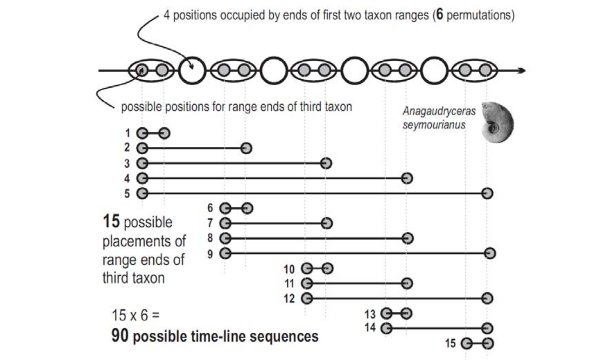
• in actuality, there are 6 different possibilities that could be considered
• time is older on the left, and younger on the right
• we can rule out some of these, because we have direct evidence of coexistence
• this is pretty tractable, and we could pretty quickly come up with a solution
  • a guiding principle is, do the MINIMUM amount of modification needed to make the ranges consistent
• OK, but what if we are dealing with THREE TAXA
  • number of possibilities grows to 90

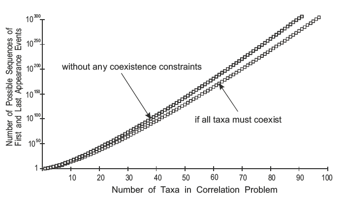
Number of possible sequences

• requires constrained optimization (CONOP9; Sadler and Cooper, 2008)
• number of atoms in universe = $10^{82}$

• quickly becomes a Herculean task, if we wanted to actually look at EVERY possible combination!
• number of atoms in universe= 10^82
• need algorithms that only look at the likliest solutions, and avoid those that can be easily discounted (called constrained opitimization)
• familiar to anyone who has played chess - 10^120 possible games

Best-fit solution

• what are some features of this that look familiar to our model outputs?

Building an age model

Building an age model

fig=plt.figure(1,figsize=(15,6))
ax=fig.add_subplot(121)
ax,trace,boxes,liths=rando_strat(ax,num_box=5,height=2,boxes=[],liths=[]) #stratigraphy for fun
#ashes in the strat column
for a in ashes: 
    tmp_w=trace[(trace[:,0]<=ashes[a]['height']) & (trace[:,1]>ashes[a]['height']),2]
    ax.plot([0,tmp_w],[ashes[a]['height'],ashes[a]['height']],'r--')
#KT boundary
tmp_w=trace[(trace[:,0]<=KT) & (trace[:,1]>KT),2]
ax.plot([0,tmp_w],[KT,KT],'k--')
ax.text(tmp_w,KT,'  KT boundary',verticalalignment='center',fontsize=20)
#ash ages
ax=fig.add_subplot(122)
for a in ashes:
    ax.plot(ashes[a]['age'],ashes[a]['height'],'rs')
ax.plot([66.2,65.95],[KT,KT],'k--')
ax.set_xlim([66.2,65.95]); ax.set_ylim([-0.1,2])
ax.set_ylabel('meters'); _=ax.set_xlabel('age (Ma)')