Lecture 13: Age models part 2
- Building an age model
- dealing with uncertainty
- Introduction to carbonates
from matplotlib.patches import Polygon
import scipy.stats as stats
from scipy.interpolate import interp1d
from matplotlib import pyplot as plt
import numpy as np
def rando_strat(ax,num_box,height,boxes,liths):
    box_colors= [('#FFB142',0.6),('#33D9B2',0.5),('#34ACE0',0.4),('#706FD3',0.3),('#2C2C54',0.2),('#84817A',0.1)]
    if len(boxes)==0:
        boxes=np.cumsum(np.random.gamma(1,1, num_box))
        boxes=boxes/boxes[-1]*height
        boxes=np.hstack((boxes[0],np.diff(boxes)))
        liths=np.random.randint(0,len(box_colors),num_box)
    stack=0
    trace=[]
    for i,s in enumerate(boxes):
        tmp_w=box_colors[liths[i]][1]
        tmp_color=box_colors[liths[i]][0]
        #add a lithostratigraphy box
        xy=np.array([(0,stack),
                     (0+tmp_w,stack),
                     (0+tmp_w,stack+s),
                     (0,stack+s)])
        rect = Polygon(xy,closed=True,
                      facecolor=tmp_color,edgecolor="k",lw=0.5)
        ax.add_patch(rect)
        #grow the net record
        trace.append((stack,stack+s,tmp_w))
        stack=stack+s
    #set y-limits (from height of this column)
    ax.set_ylim([-0.1,height+0.01*height])
    #set x-limits (section-specific max width of strat box)
    ax.set_xlim([0,1])
    #turn off axes and frame
    ax.axis('off')
    return ax,np.array(trace),boxes,liths
def calc_age(ash_table,h):
    up=ash_table[(ash_table[:,1])>h][0]
    down=ash_table[(ash_table[:,1])<h][-1]
    sed_rate=(up[1]-down[1])/(down[0]-up[0]) #[1] is height, [0] is age

    h_diff=h-down[1]
    h_age=down[0]-h_diff/sed_rate

    return(h_age)

ashes={'ash1':{'height':0.1,
            'age': 66.153,
            '2sd':0.029},
       'ash2':{'height':0.83,
            'age': 66.043,
            '2sd':0.031},
       'ash3':{'height':1.6,
            'age': 65.985,
            '2sd':0.011}}
ash_table=np.array([(ashes[a]['age'],ashes[a]['height']) for a in ashes])
KT=0.6 #height in meters
def plot_ash(boxes = [], liths = []):
    fig=plt.figure(1,figsize=(15,6))
    ax=fig.add_subplot(121)
    ax,trace,boxes,liths=rando_strat(ax,num_box=5,height=2,boxes=boxes,liths=liths) #stratigraphy for fun
    #ashes in the strat column
    for a in ashes:
        tmp_w=trace[(trace[:,0]<=ashes[a]['height']) & (trace[:,1]>ashes[a]['height']),2]
        ax.plot([0,tmp_w],[ashes[a]['height'],ashes[a]['height']],'r--')
    #KT boundary
    tmp_w=trace[(trace[:,0]<=KT) & (trace[:,1]>KT),2]
    ax.plot([0,tmp_w],[KT,KT],'k--')
    ax.text(tmp_w,KT,'  KT boundary',verticalalignment='center',fontsize=20)
    #ash ages
    ax=fig.add_subplot(122)
    for a in ashes:
        ax.plot(ashes[a]['age'],ashes[a]['height'],'rs')
    ax.plot([66.2,65.95],[KT,KT],'k--')
    ax.set_xlim([66.2,65.95]); ax.set_ylim([-0.1,2])
    ax.set_ylabel('meters'); _=ax.set_xlabel('age (Ma)')
    return boxes, liths, fig
Building an age model
boxes, liths, _ = plot_ash()

What is the age of the KT Boundary? What ages are possible? What ages are most likely?
Building an age model
Starting simple since we cant assume slow then fast is any more likely than fast then slow. Considering a constant sedimentation rate (a linear interpolation)..
_,_, fig = plot_ash(boxes=boxes,liths=liths)
#calculate KT age
ax = fig.axes[-1]
KT_age=calc_age(ash_table,KT)
ax.plot([KT_age,KT_age],[KT,KT],'w*',mec='k',markersize=20)
_=ax.text(KT_age,KT-.1,'   %2.2f Ma.' % (KT_age),horizontalalignment='left',verticalalignment='center',fontsize=20)

Even with the simple model.. what havn't we considered?
Building an age model
Starting simple since we cant assume slow then fast is any more likely than fast then slow. Considering a constant sedimentation rate (a linear interpolation)..
_,_, fig = plot_ash(boxes=boxes,liths=liths)
#calculate KT age
ax = fig.axes[-1]
KT_age=calc_age(ash_table,KT)
ax.plot([KT_age,KT_age],[KT,KT],'w*',mec='k',markersize=20)
_=ax.text(KT_age,KT-.1,'   %2.2f Ma.' % (KT_age),horizontalalignment='left',verticalalignment='center',fontsize=20)
Even with the simple model.. what havn't we considered? Uncertainty in the geochronology
Building an age model
_,_, fig = plot_ash(boxes=boxes,liths=liths)
ax = fig.axes[-1]
for a in ashes:
    ax.plot(ashes[a]['age'],ashes[a]['height'],'rs')
    ax.plot([ashes[a]['age']+ashes[a]['2sd'],ashes[a]['age']-ashes[a]['2sd']],
            [ashes[a]['height'],ashes[a]['height']],'r-')

Building an age model
_,_, fig = plot_ash(boxes=boxes,liths=liths)
ax = fig.axes[-1]
for a in ashes:
    mu=ashes[a]['age'] #normal distribution
    sigma=ashes[a]['2sd']/2
    x = np.linspace(mu - 3*sigma, mu + 3*sigma, 300)
    distro=stats.norm.pdf(x, mu, sigma) #scaled for display
    distro=distro/max(distro)*0.3
    ax.plot(x, distro+ashes[a]['height'],'r')
    #ash strat height
    ax.plot([ashes[a]['age']+ashes[a]['2sd']*3/2,ashes[a]['age']-ashes[a]['2sd']*3/2],
            [ashes[a]['height'],ashes[a]['height']],'r--',lw=0.5)

Building an age model
How do we include these normally distributed uncertainties into our constant sedimentation rate age model?
Consider..
$$ Z = (Y\pm\sigma_Y) + (X\pm\sigma_X) $$What is Z? What is $\sigma_Z$?
Building an age model
How do we include these normally distributed uncertainties into our constant sedimentation rate age model?
Consider..
$$ Z = (Y\pm\sigma_Y) + (X\pm\sigma_X) $$What is Z? (sum of the means) What is $\sigma_Z$? (square root of $\Sigma\sigma^2$)
import numpy as np
Y = np.random.normal(2,.3,1000000)
X = np.random.normal(20,.2,1000000)
Z = Y + X
print(f"""Mean of Z: {np.mean(Z):.1f} and standard deviation of Z: {np.std(Z):.2f}
Analytical stdev: {(.3**2+.2**2)**(1/2):.2f}""")
Mean of Z: 22.0 and standard deviation of Z: 0.36
Analytical stdev: 0.36
Building an age model
How do we include these normally distributed uncertainties into our constant sedimentation rate age model?
Consider..
$$ Z = (Y\pm\sigma_Y) \times (X\pm\sigma_X) $$What is Z? What is $\sigma_Z$?
Building an age model
How do we include these normally distributed uncertainties into our constant sedimentation rate age model?
Consider..
$$ Z = (Y\pm\sigma_Y) \times (X\pm\sigma_X) $$What is Z? (product of the means) What is $\sigma_Z$? (square root of the sum of the relative errors squared times mean of Z)
$$ \frac{\sigma_Z}{Z} \approx \left(\left(\frac{\sigma_Y}{Y}\right)^2 + \left(\frac{\sigma_X}{X}\right)^2\right)^\frac{1}{2} $$import numpy as np
Y = np.random.normal(2,.3,1000000)
X = np.random.normal(20,.2,1000000)
Z = Y * X
print(f"""Mean of Z: {np.mean(Z):.1f} and standard deviation of Z: {np.std(Z):.1f}
Analytical stdev: {np.mean(Z)*((0.3/2)**2+(0.2/20)**2)**(1/2):.2f}""")
Mean of Z: 40.0 and standard deviation of Z: 6.0
Analytical stdev: 6.01
Building an age model
Let's apply these rules to linear interpolation:
$$\mathrm{ \dfrac{A_{KT}-A_{0}}{H_{KT}-H_{0}}=\dfrac{A_{1}-A_{0}}{H_{1}-H_{0}}\\}$$Building an age model
Let's apply these rules to linear interpolation:
$$\mathrm{ \dfrac{A_{KT}-A_{0}}{H_{KT}-H_{0}}=\dfrac{A_{1}-A_{0}}{H_{1}-H_{0}}\\ A_{KT}=\left(\dfrac{A_{1}-A_{0}}{H_{1}-H_{0}}\right)(H_{KT}-H_{0})+A_{0}\\ }$$Building an age model
Let's apply these rules to linear interpolation:
$$\mathrm{ \dfrac{A_{KT}-A_{0}}{H_{KT}-H_{0}}=\dfrac{A_{1}-A_{0}}{H_{1}-H_{0}}\\ A_{KT}=\left(\dfrac{A_{1}-A_{0}}{H_{1}-H_{0}}\right)(H_{KT}-H_{0})+A_{0}\\ A_{KT}=\left(\dfrac{\color{red}{A_{1}-A_{0}}}{H_{1}-H_{0}}\right)(H_{KT}-H_{0})+\color{red}{A_{0}}\\ } $$Building an age model
Let's apply these rules to linear interpolation:
$$\mathrm{ \dfrac{A_{KT}-A_{0}}{H_{KT}-H_{0}}=\dfrac{A_{1}-A_{0}}{H_{1}-H_{0}}\\ A_{KT}=\left(\dfrac{A_{1}-A_{0}}{H_{1}-H_{0}}\right)(H_{KT}-H_{0})+A_{0}\\ A_{KT}=\left(\dfrac{\color{red}{A_{1}-A_{0}}}{H_{1}-H_{0}}\right)(H_{KT}-H_{0})+\color{red}{A_{0}}\\ \\ \sigma A_{kt}^2=\left((\sigma A_{0}^2 + \sigma A_{1}^2)^\frac{1}{2}\times\frac{H_{KT}-H_{0}}{H_{1}-H_{0}}\right)^2 + \sigma A_{0}^2}$$age = (
lambda ashes, ktH: (ashes["ash2"]["age"] - ashes["ash1"]["age"])
/ (ashes["ash2"]["height"] - ashes["ash1"]["height"])
* (ktH - ashes["ash1"]["height"])
+ ashes["ash1"]["age"]
)
draws = []
for i in range(10000):
    simulated_ash = {
        "ash1": {
            "height": 0.1,
            "age": np.random.normal(66.153, 0.029 / 2),
            "2sd": 0.029,
        },
        "ash2": {
            "height": 0.83,
            "age": np.random.normal(66.043, 0.031 / 2),
            "2sd": 0.031,
        },
        "ash3": {
            "height": np.random.normal(66.153, 0.011 / 2),
            "age": 65.985,
            "2sd": 0.011,
        },
    }
    draws.append(age(simulated_ash, KT))
print(np.std(draws))
0.011619603147695575
plt.figure(figsize=(8,8))
a1 = np.random.normal(66.153, 0.029 * 2, 10000)
a2 = np.random.normal(66.043, 0.031 * 2, 10000)
plt.plot(a1,a2,'.',alpha=.3)
plt.gca().set_aspect('equal')
plt.gca().set_xlabel('Lower ash age')
plt.gca().set_ylabel('Upper ash age')
Text(0, 0.5, 'Upper ash age')

plt.figure(figsize=(8, 8))
a1 = np.random.normal(66.153, 0.029 * 2, 10000)
a2 = np.random.normal(66.043, 0.031 * 2, 10000)
plt.plot(a1, a2, ".", alpha=0.3)
plt.plot(a1[a1 < a2], a2[a1 < a2], "r.", alpha=0.1)
plt.gca().set_aspect("equal")
plt.gca().set_xlabel("Lower ash age")
plt.gca().set_ylabel("Upper ash age")
Text(0, 0.5, 'Upper ash age')

Building an age model
How do we include these normally distributed uncertainties into our constant sedimentation rate age model?
- Even in our simple model the uncertainty is not exactly normal (there is covariation)
- Random number generators allow us account to account for these more complicated forms of uncertainty (Monte Carlo methods)
Power of Monte Carlo approaches
How many samples is enough?
fig=plt.figure(1,figsize=(15,6))
ax=fig.add_subplot(111)
idx=list(range(1000)) +list(range(1000,len(KT_ages)+1,100))
#statistics of KT age as function of number of trials
KT_evolve=[]
for i in idx[:10000]: #more trials here
    KT_evolve.append((np.mean(KT_ages[0:i+1]),np.std(KT_ages[0:i+1]),len(KT_ages[0:i+1])))
KT_evolve=np.array(KT_evolve)
#plot the results
ax.plot(KT_evolve[:,2],KT_evolve[:,0],'r-',label='mean age')
ax.fill_between(KT_evolve[:,2],KT_evolve[:,0]+KT_evolve[:,1],KT_evolve[:,0]-KT_evolve[:,1],
                color='k',alpha=0.5,zorder=0,label='mean +/- 2s.d.')
ax.set_ylabel('age (Ma.)'); ax.set_xlabel('number of trials');_=ax.legend(loc='best')

Constant sedimentation rate assumption
def make_path(pts,g_shape,g_scale,delta):
    #separate a number of points (X) along a [0,1] path
    if pts!=0:
        #X numbers are drawn from a gamma distribution (G)
        #--> these represent the distances between successive points
        path=np.cumsum(np.random.gamma(g_shape,g_scale, pts))
    else:
        path=[1]#if X = 0, then path is simply [0,1]
    path=np.hstack((0,path))#add 0 as the path beginning
    #scale first to be between 0 and 1, and then 0 to delta
    path=path/path[-1]*delta
    return(path)

fig=plt.figure(1,figsize=(6,6)); ax=fig.add_subplot(111)
#assumes constant sedimentation rate between anchors
ax.plot([0,1],[0,1],'-s');ax.set_xlabel('change in time'); _=ax.set_ylabel('change in height')

Constant sedimentation rate assumption
- goal in lab tomorrow: how can we get away from the assumption of constant sedimentation rate? what should it look like?
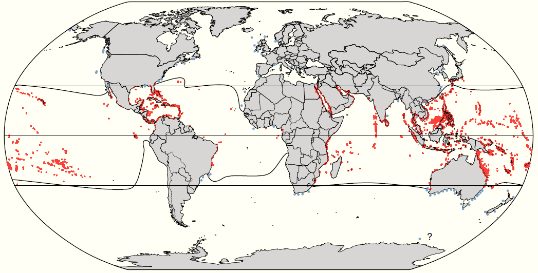
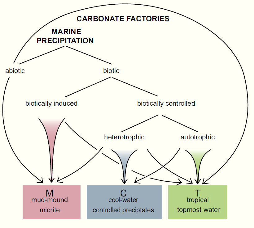
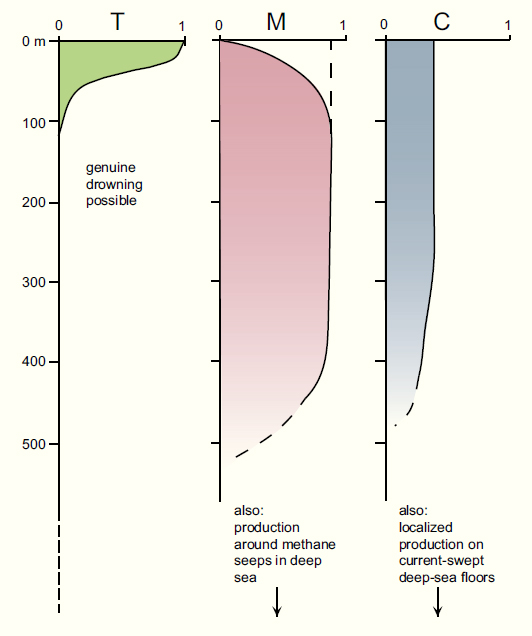
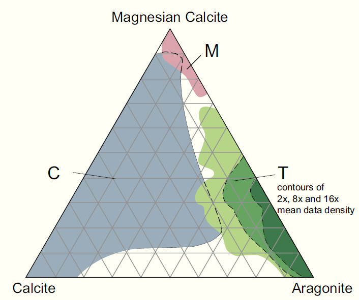
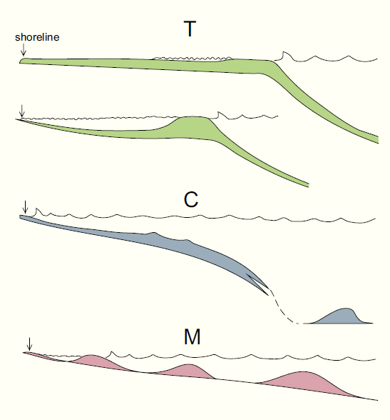
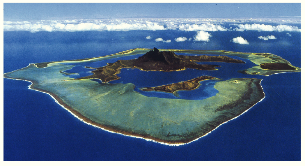
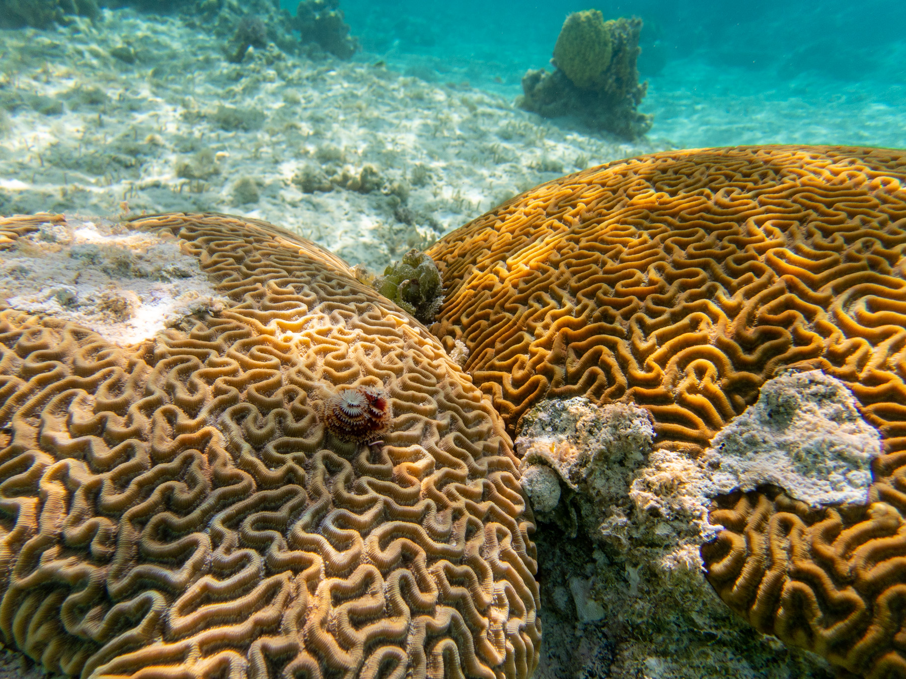
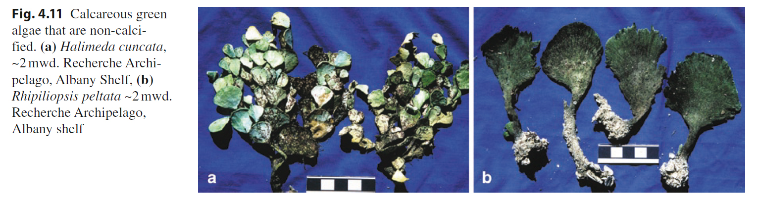
Carbonates